![]()
![]()
![]()
Search and download data from the Swiss Federal Statistical Office
The BFS package allows to search and download public
data from the
Swiss Federal Statistical Office (BFS stands for
Bundesamt für Statistik in German) APIs in a dynamic and
reproducible way.
install.packages("BFS")You can also install the development version from Github.
devtools::install_github("lgnbhl/BFS")library(BFS)To get data from the Swiss Stats
Explorer API (SSE) you first create a query using the metadata
codelist from SSE using the bfs_get_sse_metadata()
function. First get the codelist of a BFS dataset:
codelist <- bfs_get_sse_metadata("DF_LWZ_1", language = "en")

codelist
## # A tibble: 2,321 × 5
## code text value valueText position_dimension
## <chr> <chr> <chr> <chr> <int>
## 1 GR_KT_GDE Cantons, districts and municipa… 1 Aeugst a… 1
## 2 GR_KT_GDE Cantons, districts and municipa… 10 Obfelden 1
## 3 GR_KT_GDE Cantons, districts and municipa… 100 Stadel 1
## 4 GR_KT_GDE Cantons, districts and municipa… 1001 Dopplesc… 1
## 5 GR_KT_GDE Cantons, districts and municipa… 1002 Entlebuch 1
## 6 GR_KT_GDE Cantons, districts and municipa… 1004 Flühli 1
## 7 GR_KT_GDE Cantons, districts and municipa… 1005 Hasle (L… 1
## 8 GR_KT_GDE Cantons, districts and municipa… 1007 Romoos 1
## 9 GR_KT_GDE Cantons, districts and municipa… 1008 Schüpfhe… 1
## 10 GR_KT_GDE Cantons, districts and municipa… 1009 Werthens… 1
## # ℹ 2,311 more rowsThen filter the codelist to build your query:
querydat <- codelist %>%
  dplyr::filter((code == "GR_KT_GDE" & valueText %in% c("Aarau", "Olten")) |
                  (code == "WOHN_ANZAHL" & valueText == "Total") |
                  (code == "LEERWOHN_TYP" & valueText == "Vacant dwelling for rent") |
                  (code == "MEASURE_DIMENSION" & valueText == "Value"))
query <- tapply(querydat$value, querydat$code, c)

query
## $GR_KT_GDE
## [1] "2581" "4001"
##
## $LEERWOHN_TYP
## [1] "4"
##
## $MEASURE_DIMENSION
## [1] "V"
##
## $WOHN_ANZAHL
## [1] "_T"This query can be used in the new bfs_get_sse_data()
function to import the data.
bfs_get_sse_data(
  number_bfs = "DF_LWZ_1",
  language = "en",
  query =  query,
  start_period = "2020",
  end_period = "2023"
)
## # A tibble: 8 × 7
## TIME_PERIOD GR_KT_GDE WOHN_ANZAHL LEERWOHN_TYP MEASURE_DIMENSION FREQ value
## <chr> <chr> <chr> <chr> <chr> <chr> <dbl>
## 1 2020 Olten Total Vacant dwelli… Value Annu… 350
## 2 2021 Olten Total Vacant dwelli… Value Annu… 393
## 3 2022 Olten Total Vacant dwelli… Value Annu… 418
## 4 2023 Olten Total Vacant dwelli… Value Annu… 266
## 5 2020 Aarau Total Vacant dwelli… Value Annu… 110
## 6 2021 Aarau Total Vacant dwelli… Value Annu… 85
## 7 2022 Aarau Total Vacant dwelli… Value Annu… 61
## 8 2023 Aarau Total Vacant dwelli… Value Annu… 49Before downloading a BFS dataset, you need to get its related BFS
number (FSO number) in the official
data catalog. You can search in the catalog directly from R using
the bfs_get_catalog_data() function in any language (“de”,
“fr”, “it” or “en”):
bfs_get_catalog_data(language = "en", extended_search = "student")## # A tibble: 4 × 6
## title language number_bfs number_asset publication_date url_px
## <chr> <chr> <chr> <chr> <date> <chr>
## 1 University of applie… en px-x-1502… 34248852 2025-03-27 https…
## 2 University of applie… en px-x-1502… 34248849 2025-03-27 https…
## 3 University students … en px-x-1502… 34248664 2025-03-27 https…
## 4 University students … en px-x-1502… 34248666 2025-03-27 https…You can search in the data catalog using the following arguments:
language: The language of a BFS catalog, i.e. “de”,
“fr”, “it” or “en”.title: to search in title, subtitle and
supertitle.extended_search: extended search in (sub/super)title,
orderNr, summary, shortSummary, shortTextGNP.spatial_division: choose between “Switzerland”,
“Cantons”, “Districts”, “Communes”, “Other spatial divisions” or
“International”.prodima: by specific BFS themes using a unique prodima
number.inquiry: by inquiry number.institution: by institution.publishing_year_start: by publishing year start.publishing_year_end: by publishing year end.order_nr: by BFS Number (FSO number).limit: limit of query results (API limit seems to be
350)article_model_group: article model grouparticle_model: article modelNote that English (“en”) and Italian (“it”) data catalogs offer a
limited list of datasets. For the full list please get the French (“fr”)
or German (“de”) data catalogs (see language_available
column).
To return all the catalog metadata in the raw (uncleaned) structure,
you can add return_raw = TRUE:
catalog_raw <- bfs_get_catalog_data(
  language = "en",
  extended_search = "student",
  return_raw = TRUE
)

catalog_raw
## # A tibble: 4 × 5
## ids$uuid $contentId bfs$embargo description$titles$m…¹ shop$orderNr links
## <chr> <int> <chr> <chr> <chr> <lis>
## 1 1e58cdb7-01b… 2301224 2025-03-27… University of applied… px-x-150204… <df>
## 2 fa6d167c-6b6… 2301215 2025-03-27… University of applied… px-x-150204… <df>
## 3 dfd53d00-f5c… 2301207 2025-03-27… University students b… px-x-150204… <df>
## 4 8f4fb90d-b6a… 2301195 2025-03-27… University students b… px-x-150204… <df>
## # ℹ abbreviated name: ¹description$titles$main
## # ℹ 14 more variables: ids$gnp <chr>, $damId <int>, $languageCopyId <int>,
## # bfs$lifecycle <df[,4]>, $lifecycleGroup <chr>, $provisional <lgl>,
## # $articleModel <df[,4]>, $articleModelGroup <df[,4]>,
## # description$categorization <df[,13]>, $bibliography <df[,1]>,
## # $shortSummary <df[,2]>, $language <chr>, $abstractShort <chr>,
## # shop$stock <lgl>The data catalog in a raw structure returns a data.frame containing
nested data.frames in some columns. Here an example to get the
description nested data.frame as a tibble:
library(dplyr)

as_tibble(catalog_raw$description)
## # A tibble: 4 × 6
## titles$main categorization$colle…¹ bibliography$period shortSummary$html
## <chr> <list> <chr> <chr>
## 1 University of ap… <df [2 × 4]> 1997-2024 This dataset pre…
## 2 University of ap… <df [2 × 4]> 1997-2024 This dataset pre…
## 3 University stude… <df [2 × 4]> 1990-2024 This dataset pre…
## 4 University stude… <df [2 × 4]> 1980-2024 This dataset pre…
## # ℹ abbreviated name: ¹categorization$collection
## # ℹ 15 more variables: categorization$prodima <list>, $inquiry <list>,
## # $spatialdivision <list>, $classification <list>, $institution <list>,
## # $publisher <list>, $tags <list>, $dataSource <list>, $copyrights <list>,
## # $termsOfUse <list>, $serie <list>, $periodicity <list>,
## # shortSummary$raw <chr>, language <chr>, abstractShort <chr>As the API limit is 350 results, you can get the full data catalog by
looping on specific parameters. For example, you can loop over all
prodima numbers (equivalent to BFS themes):
# themes_names <- c("Statistical basis and overviews 00", "Population 01", "Territory and environment 02", "Work and income 03", "National economy 04", "Prices 05", "Industry and services 06", "Agriculture and forestry 07", "Energy 08", "Construction and housing 09", "Tourism 10", "Mobility and transport 11", "Money, banks and insurance 12", "Social security 13", "Health 14", "Education and science 15", "Culture, media, information society, sports 16", "Politics 17", "General Government and finance 18", "Crime and criminal justice 19", "Economic and social situation of the population 20", "Sustainable development, regional and international disparities 21")
themes_prodima <- c(900001, 900010, 900035, 900051, 900075, 900084, 900092, 900104, 900127, 900140, 900160, 900169, 900191, 900198, 900210, 900212, 900214, 900226, 900239, 900257, 900269, 900276)

library(purrr)

catalog_all <- purrr::pmap_dfr(
  .l = list(language = "de", prodima = themes_prodima, return_raw = TRUE),
  .f = bfs_get_catalog_data,
)

catalog_all
## # A tibble: 768 × 5
## ids$uuid $contentId bfs$embargo description$titles$m…¹ shop$orderNr links
## <chr> <int> <chr> <chr> <chr> <lis>
## 1 c001d7d3-c8… 325772 2025-09-25… Heiraten und Heiratsh… px-x-010202… <df>
## 2 be1f72da-ab… 189095 2025-09-25… Lebendgeburten nach M… px-x-010202… <df>
## 3 595d7bde-97… 325776 2025-09-25… Scheidungen und Schei… px-x-010202… <df>
## 4 cbc06e96-d8… 189065 2025-09-25… Todesfälle nach Monat… px-x-010202… <df>
## 5 ed95f4e3-4a… 13807205 2025-08-28… Männliche Vornamen de… px-x-010405… <df>
## 6 dcefda9c-b6… 13807212 2025-08-28… Weibliche Vornamen de… px-x-010405… <df>
## 7 4d53b847-9d… 189124 2025-08-27… Auswanderung der stän… px-x-010302… <df>
## 8 010ce6b9-38… 189120 2025-08-27… Auswanderung der stän… px-x-010302… <df>
## 9 baf1b850-e1… 189087 2025-08-27… Auswanderung der stän… px-x-010302… <df>
## 10 a3460776-11… 325764 2025-08-27… Auswanderung der stän… px-x-010302… <df>
## # ℹ 758 more rows
## # ℹ abbreviated name: ¹description$titles$main
## # ℹ 16 more variables: ids$gnp <chr>, $damId <int>, $languageCopyId <int>,
## # bfs$lifecycle <df[,4]>, $lifecycleGroup <chr>, $provisional <lgl>,
## # $articleModel <df[,4]>, $articleModelGroup <df[,4]>,
## # $lastUpdatedVersion <chr>, description$titles$sub <chr>,
## # description$categorization <df[,13]>, $bibliography <df[,2]>, …# to not overload the server, please save the data frame locally
# readr::write_csv(catalog_all, "catalog_all.csv")
# catalog_all <- readr::read_csv("catalog_all.csv") Please use this loop moderately to not overload BFS server unnecessarily (just run it when needed and save the result locally).
The function bfs_get_data() allows you to download any
dataset from the BFS
catalog (equivalent to selecting “data” in the “Article Type”
dropdown of the BFS website) using its BFS number (FSO number).
Using the number_bfs argument (FSO number), you can get
BFS data in a given language (“en”, “de”, “fr” or “it”) from the
official PXWeb API of the Swiss Federal Statistical Office.
#catalog_student$number_bfs[1] # px-x-1502040100_131
bfs_get_data(number_bfs = "px-x-1502040100_131", language = "en")
## # A tibble: 18,900 × 5
## Year `ISCED Field` Sex `Level of study` `University students`
## <chr> <chr> <chr> <chr> <dbl>
## 1 1980/81 Education science Male First university degr… 545
## 2 1980/81 Education science Male Bachelor 0
## 3 1980/81 Education science Male Master 0
## 4 1980/81 Education science Male Doctorate 93
## 5 1980/81 Education science Male Further education, ad… 13
## 6 1980/81 Education science Female First university degr… 946
## 7 1980/81 Education science Female Bachelor 0
## 8 1980/81 Education science Female Master 0
## 9 1980/81 Education science Female Doctorate 70
## 10 1980/81 Education science Female Further education, ad… 52
## # ℹ 18,890 more rowsWhen running the bfs_get_data() function you may get the
following error message (issue #7).
Error in pxweb_advanced_get(url = url, query = query, verbose = verbose) :
  Too Many Requests (RFC 6585) (HTTP 429).
This could happen because you ran too many times a
bfs_get_*() function (API config is here). A
solution is to wait a few seconds before running the next
bfs_get_*() function. You can add a delay in your R code
using the delay argument.
bfs_get_data(
  number_bfs = "px-x-1502040100_131",
  language = "en",
  delay = 10
)
If the error message remains, it could be because you are querying a
very large BFS dataset. Two workarounds exist: a) download the BFS file
using bfs_download_asset() to read it locally or b) query
only specific elements of the data to reduce the API call (see next
section).
Here an example using the bfs_download_asset()
function:
BFS::bfs_download_asset(
  number_bfs = "px-x-1502040100_131", #number_asset also possible
  destfile = "px-x-1502040100_131.px"
)

library(pxR) # install.packages("pxR")
large_dataset <- pxR::read.px(filename = "px-x-1502040100_131.px") |>
  as.data.frame()
Note that reading a PX file using pxR::read.px() gives
access only to the German version.
First you want to get the metadata of your dataset, i.e. the
variables (code and text) and dimensions
(values and valueTexts). For example:
metadata <- bfs_get_metadata(number_bfs = "px-x-1502040100_131", language = "en")

# tidy metadata
library(dplyr)
library(tidyr) # for unnest_longer

metadata_tidy <- metadata |>
  unnest_longer(c(values, valueTexts))

metadata_tidy
## # A tibble: 92 × 7
## code text values valueTexts time elimination
## <chr> <chr> <chr> <chr> <lgl> <lgl>
## 1 Jahr Year 0 1980/81 TRUE NA
## 2 Jahr Year 1 1981/82 TRUE NA
## 3 Jahr Year 2 1982/83 TRUE NA
## 4 Jahr Year 3 1983/84 TRUE NA
## 5 Jahr Year 4 1984/85 TRUE NA
## 6 Jahr Year 5 1985/86 TRUE NA
## 7 Jahr Year 6 1986/87 TRUE NA
## 8 Jahr Year 7 1987/88 TRUE NA
## 9 Jahr Year 8 1988/89 TRUE NA
## 10 Jahr Year 9 1989/90 TRUE NA
## # ℹ 82 more rows
## # ℹ 1 more variable: title <chr>Then you can filter the dimensions you want to query using the
text and valueTexts variables and build the
query dimension object with the code and
values variables.
# select dimensions
dim1 <- metadata_tidy |>
  filter(text == "Year" & valueTexts %in% c("2020/21", "2021/22"))
dim2 <- metadata_tidy |>
  filter(text == "Level of study" & valueTexts %in% c("Master", "Doctorate"))
dim3 <- metadata_tidy |>
  filter(text == "ISCED Field" & valueTexts %in% c("Education science"))
dim4 <- metadata_tidy |>
  filter(text == "Sex") # all valueTexts dimensions

# build dimensions list object
dimensions <- list(
  dim1$values,
  dim2$values,
  dim3$values,
  dim4$values
)

names(dimensions) <- c(
  unique(dim1$code),
  unique(dim2$code),
  unique(dim3$code),
  unique(dim4$code)
)

dimensions
## $Jahr
## [1] "40" "41"
##
## $Studienstufe
## [1] "2" "3"
##
## $`ISCED Fach`
## [1] "0"
##
## $Geschlecht
## [1] "0" "1"Finally you can query BFS data with specific dimensions.
BFS::bfs_get_data(
  number_bfs = "px-x-1502040100_131",
  language = "en",
  query = dimensions
  )
## # A tibble: 8 × 5
## Year `ISCED Field` Sex `Level of study` `University students`
## <chr> <chr> <chr> <chr> <dbl>
## 1 2020/21 Education science Male Master 151
## 2 2020/21 Education science Male Doctorate 121
## 3 2020/21 Education science Female Master 555
## 4 2020/21 Education science Female Doctorate 306
## 5 2021/22 Education science Male Master 143
## 6 2021/22 Education science Male Doctorate 115
## 7 2021/22 Education science Female Master 599
## 8 2021/22 Education science Female Doctorate 318A lot of datasets are not accessible through the official PXWeb API.
They are listed in the data
catalog as “tables” in the “Article Type” dropdown of the BFS
website. You can search for specific tables using
bfs_get_catalog_tables().
catalog_tables_en_students <- bfs_get_catalog_tables(language = "en", extended_search = "students")

catalog_tables_en_students
## # A tibble: 5 × 5
## title language number_asset publication_date order_nr
## <chr> <chr> <chr> <date> <chr>
## 1 Students at universities and … en 35008068 2025-03-27 ts-x-15…
## 2 Students at universities and … en 34707698 2025-03-27 su-e-15…
## 3 Students at universities of a… en 35008067 2025-03-27 ts-x-15…
## 4 Students at universities of a… en 34707700 2025-03-27 su-e-15…
## 5 Students at universities of t… en 34707695 2025-03-27 su-e-15…Most of the BFS tables are Excel or CSV files. You can download an
table with bfs_download_asset() using the
number asset.
library(dplyr)

tables_asset_number_students <- catalog_tables_en_students |>
  dplyr::filter(title == "Students at universities and institutes of technology: Basistables") |>
  dplyr::pull(number_asset)

file_path <- BFS::bfs_download_asset(
  number_asset = tables_asset_number_students,
  destfile = "su-e-15.02.04.01.xlsx"
)
To return all the catalog metadata in the raw (uncleaned) structure,
you can add return_raw = TRUE:
catalog_tables_raw <- bfs_get_catalog_tables(
  language = "en",
  extended_search = "student",
  return_raw = TRUE
)

catalog_tables_raw
## # A tibble: 6 × 5
## ids$uuid $contentId bfs$embargo description$titles$m…¹ shop$orderNr links
## <chr> <int> <chr> <chr> <chr> <lis>
## 1 2f0d3744-3b1… 14876281 2025-10-27… Student mobility with… su-e-15.02.… <df>
## 2 bf5e392a-e95… 20044168 2025-03-27… Students at universit… ts-x-15.02.… <df>
## 3 c9eb6b70-43f… 528179 2025-03-27… Students at universit… su-e-15.02.… <df>
## 4 36a042c8-b94… 20044200 2025-03-27… Students at universit… ts-x-15.02.… <df>
## 5 28ce8307-668… 528173 2025-03-27… Students at universit… su-e-15.02.… <df>
## 6 d3bc2d74-119… 528176 2025-03-27… Students at universit… su-e-15.02.… <df>
## # ℹ abbreviated name: ¹description$titles$main
## # ℹ 14 more variables: ids$gnp <chr>, $damId <int>, $languageCopyId <int>,
## # bfs$lifecycle <df[,4]>, $lifecycleGroup <chr>, $provisional <lgl>,
## # $articleModel <df[,4]>, $articleModelGroup <df[,4]>,
## # description$categorization <df[,13]>, $bibliography <df[,1]>,
## # $language <chr>, $shortSummary <df[,2]>, $abstractShort <chr>,
## # shop$stock <lgl>The data catalog in a raw structure returns a data.frame containing
nested data.frames in some columns. Here an example to get the
description nested data.frame as a tibble:
library(dplyr)

as_tibble(catalog_tables_raw$description)
## # A tibble: 6 × 6
## titles$main categorization$colle…¹ bibliography$period language
## <chr> <list> <chr> <chr>
## 1 Student mobility within S… <df [2 × 4]> 2023 EN
## 2 Students at universities … <df [3 × 4]> 1980-2024 DE/EN/F…
## 3 Students at universities … <df [3 × 4]> 1990-2024 EN
## 4 Students at universities … <df [3 × 4]> 2000-2024 DE/EN/F…
## 5 Students at universities … <df [3 × 4]> 1997-2024 EN
## 6 Students at universities … <df [2 × 4]> 2005-2024 EN
## # ℹ abbreviated name: ¹categorization$collection
## # ℹ 14 more variables: categorization$prodima <list>, $inquiry <list>,
## # $spatialdivision <list>, $classification <list>, $institution <list>,
## # $publisher <list>, $tags <list>, $dataSource <list>, $copyrights <list>,
## # $termsOfUse <list>, $serie <list>, $periodicity <list>,
## # shortSummary <df[,2]>, abstractShort <chr>Display geo-information catalog of the Swiss Official STAC API using
bfs_get_catalog_geodata().
library(rstac) # install.packages("rstac")

catalog_geodata <- bfs_get_catalog_geodata(include_metadata = TRUE)

catalog_geodata
## # A tibble: 281 × 12
## collection_id type href title description created updated crs license
## <chr> <chr> <chr> <chr> <chr> <chr> <chr> <chr> <chr>
## 1 ch.are.agglomera… API http… Citi… "The list … 2021-1… 2023-0… http… propri…
## 2 ch.are.alpenkonv… API http… Alpi… "The perim… 2021-1… 2022-0… http… propri…
## 3 ch.are.belastung… API http… Load… "Passenger… 2021-1… 2022-0… http… propri…
## 4 ch.are.belastung… API http… Load… "Passenger… 2021-1… 2022-0… http… propri…
## 5 ch.are.belastung… API http… Load… "Vehicles … 2021-1… 2022-0… http… propri…
## 6 ch.are.belastung… API http… Load… "Vehicles … 2021-1… 2022-0… http… propri…
## 7 ch.are.erreichba… API http… Acce… "Accessibi… 2021-1… 2022-0… http… propri…
## 8 ch.are.erreichba… API http… Acce… "Accessibi… 2021-1… 2022-0… http… propri…
## 9 ch.are.gemeindet… API http… Typo… "The typol… 2021-1… 2022-0… http… propri…
## 10 ch.are.gueteklas… API http… Publ… "The publi… 2021-1… 2023-0… http… propri…
## # ℹ 271 more rows
## # ℹ 3 more variables: provider_name <chr>, bbox <list>, inverval <list>For example you can get information about the dataset “Generalised borders G1 and area with urban character”.
library(dplyr)

geodata_g1 <- catalog_geodata |>
  filter(title == "Generalised borders G1 and area with urban character")

geodata_g1
## # A tibble: 1 × 12
## collection_id type href title description created updated crs license
## <chr> <chr> <chr> <chr> <chr> <chr> <chr> <chr> <chr>
## 1 ch.bfs.generalisi… API http… Gene… Administra… 2022-0… 2023-0… http… propri…
## # ℹ 3 more variables: provider_name <chr>, bbox <list>, inverval <list>Download dataset by collection id with
bfs_download_geodata() and unzip file if needed.
# Access Generalised borders G1 and area with urban character
borders_g1_path <- bfs_download_geodata(
  collection_id = "ch.bfs.generalisierte-grenzen_agglomerationen_g1",
  output_dir = tempdir() #  temporary directory
)

# you may need to unzip the file
unzip(borders_g1_path[4], exdir = "borders_G1")
By default, the files are downloaded in a temporary directory. You
can specify the folder where saving the files using the
output_dir argument.
Some layers are accessible using WMS (Web Map Service):
library(leaflet)

leaflet() %>%
  setView(lng = 8, lat = 46.8, zoom = 8) %>%
  addWMSTiles(
    baseUrl = "https://wms.geo.admin.ch/?",
    layers = "ch.bfs.generalisierte-grenzen_agglomerationen_g2",
    options = WMSTileOptions(format = "image/png", transparent = TRUE),
    attribution = "Generalised borders G1 © 2024 BFS")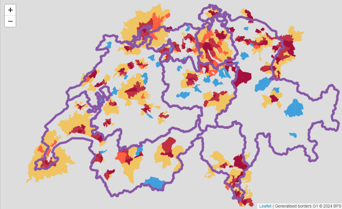
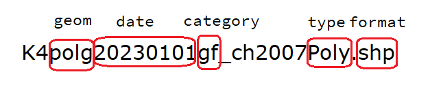
You can get cartographic
base maps from the ThemaKart project using
bfs_get_base_maps(). The list of available geometries in
the official
documentation.
The default arguments of bfs_get_base_maps() can be
change to access specific files:
library(sf) install.packages("sf")

# default arguments
bfs_get_base_maps(
  geom = NULL,
  category = "gf", # "gf" for total area (i.e. "Gesamtflaeche")
  type = "Poly",
  date = NULL,
  most_recent = TRUE, #get most recent file by default
  format = "shp",
  asset_number = "24025646" #change ThemaKart geodata as updated every year
)
A typical base maps ThemaKart file looks like this:
All available geometry files in ThemaKart asset can be listed using
return_sf = FALSE:
all_themakart_files <- bfs_get_base_maps(
  return_sf = FALSE, # do NOT return sf object
  asset_number = "30566934", # ThemaKart asset of 2024
  geom = "",
  category = "",
  type = "",
  format = "",
  date = ""
)

length(all_themakart_files) # number of files available
## [1] 701For example, all available river files can be found with:
all_river_files <- bfs_get_base_maps(
    return_sf = FALSE, # do NOT return sf object
    asset_number = "30566934", # ThemaKart asset of 2024
    geom = "flus", # "flus" for river related files
    category = "",
    type = "",
    format = "shp",
    date = ""
)
The function bfs_get_base_maps() eases file selection
with arguments and returns an sf object by default.
switzerland_sf <- bfs_get_base_maps(geom = "suis")
communes_sf <- bfs_get_base_maps(geom = "polg")
districts_sf <- bfs_get_base_maps(geom = "bezk")
cantons_sf <- bfs_get_base_maps(geom = "kant")
cantons_capitals_sf <- bfs_get_base_maps(geom = "stkt", type = "Pnts", category = "kk")
lakes_sf <- bfs_get_base_maps(geom = "seen", category = "11")
# for some reason rivers don't have a "type" in their file names, so add type = ""
rivers_sf <- bfs_get_base_maps(geom = "flus", type = "", category = "22")

library(ggplot2)

ggplot() +
  geom_sf(data = communes_sf, fill = "snow", color = "grey45") +
  geom_sf(data = lakes_sf, fill = "lightblue2", color = "black") +
  geom_sf(data = districts_sf, fill = "transparent", color = "grey65") +
  geom_sf(data = cantons_sf, fill = "transparent", color = "black") +
  geom_sf(data = rivers_sf, color = "lightblue2", lwd = 1) +
  geom_sf(data = cantons_capitals_sf, shape = 18, size = 3) +
  theme_minimal() +
  theme(axis.text = element_blank()) +
  labs(caption = "Source: ThemaKart, © BFS")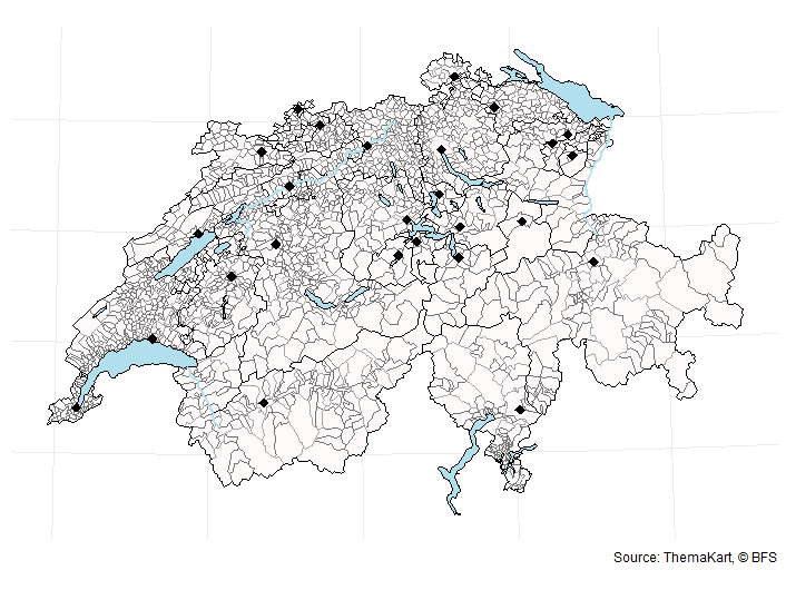
Note that the geometries are available for different date of data
release. By default, bfs_get_base_maps() tries to get the
most recent date. You can specify the date using the “date”
argument.
You can create an interactive map easily with the mapview R package.
library(mapview)

BFS::bfs_get_base_maps(geom = "bezk") |>
  mapview(zcol = "name", legend = FALSE)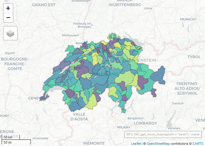
You can also get the historicized list of Swiss municipalities from the official BFS API using the new swissMunicipalities R package. The documentation is here.
# remotes::install_github("SwissStatsR/swissMunicipalities")
library(swissMunicipalities)
library(dplyr) # just for data wrangling

# snapshot of today list of Swiss municipalites/districts/cantons
snapshot <- swissMunicipalities::get_snapshots(hist_id = TRUE)

municipalities <- snapshot |>
  filter(Level == 3) |>
  rename_with(~ paste0(.x, "_municipality", recycle0 = TRUE)) |>
  select(-Level_municipality)

districts <- snapshot |>
  filter(Level == 2) |>
  rename_with(~ paste0(.x, "_district", recycle0 = TRUE)) |>
  select(-Level_district)

cantons <- snapshot |>
  filter(Level == 1) |>
  rename_with(~ paste0(.x, "_canton", recycle0 = TRUE)) |>
  select(-Level_canton)

# consolidate municipality data with districts and cantons levels
municipalities_consolidated <- municipalities |>
  left_join(districts, by = join_by(Parent_municipality == Identifier_district)) |>
  left_join(cantons, by = join_by(Parent_district == Identifier_canton)) |>
  rename(Identifier_district = Parent_municipality, Identifier_canton = Parent_district) |>
  select(starts_with(c("Identifier", "Name", "ABBREV", "Valid")), everything()) |>
  arrange(Identifier_municipality, Identifier_district)

municipalities_consolidated
# A tibble: 2,131 × 82
Identifier_municipality Identifier_district Identifier_canton Name_en_municipality Name_fr_municipality
<dbl> <dbl> <dbl> <chr> <chr>
1 1 101 1 Aeugst am Albis Aeugst am Albis
2 2 101 1 Affoltern am Albis Affoltern am Albis
3 3 101 1 Bonstetten Bonstetten
4 4 101 1 Hausen am Albis Hausen am Albis
5 5 101 1 Hedingen Hedingen
6 6 101 1 Kappel am Albis Kappel am Albis
7 7 101 1 Knonau Knonau
8 8 101 1 Maschwanden Maschwanden
9 9 101 1 Mettmenstetten Mettmenstetten
10 10 101 1 Obfelden Obfelden
# ℹ 2,121 more rows
# ℹ 77 more variables: Name_de_municipality <chr>, Name_it_municipality <chr>, Name_en_district <chr>,
# Name_fr_district <chr>, Name_de_district <chr>, Name_it_district <chr>, Name_en_canton <chr>,
# Name_fr_canton <chr>, Name_de_canton <chr>, Name_it_canton <chr>, ABBREV_1_Text_en_municipality <chr>,
# ABBREV_1_Text_fr_municipality <chr>, ABBREV_1_Text_de_municipality <chr>, ABBREV_1_Text_it_municipality <chr>,
# ABBREV_1_Text_municipality <chr>, ABBREV_1_Text_en_district <chr>, ABBREV_1_Text_fr_district <chr>,
# ABBREV_1_Text_de_district <chr>, ABBREV_1_Text_it_district <chr>, ABBREV_1_Text_district <chr>, …
# ℹ Use `print(n = ...)` to see more rowsYou can now use the consolidated list of Swiss municipalities to ease geodata analysis.
library(sf)
library(ggplot2)

communes_sf <- bfs_get_base_maps(geom = "polg", date = "20230101")

communes_ge <- communes_sf |>
  inner_join(municipalities_consolidated |>
               filter(Name_de_canton == "Genève"),
             by = c("id" = "Identifier_municipality"))

bbox_ge <- sf::st_bbox(communes_ge)

lake_leman <- bfs_get_base_maps(geom = "seen", category = "11") |>
  filter(name == "Lac Léman")

communes_ge |>
  ggplot() +
  geom_sf(data = lake_leman, fill = "lightblue2", color = "grey65") +
  geom_sf(fill = "snow", color = "grey65") +
  geom_sf_text(aes(label = name), size = 3, check_overlap = T) +
  # bounding box
  coord_sf(
    xlim = c(bbox_ge$xmin, bbox_ge$xmax),
    ylim = c(bbox_ge$ymin, bbox_ge$ymax)
  ) +
  theme_minimal() +
  theme(axis.text = element_blank()) +
  labs(title = "Communes du canton de Genève",
       x = NULL, y = NULL,
       caption = "Source: ThemaKart, © BFS")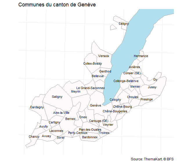
Under the hood, this package is using the pxweb package to query the Swiss Federal Statistical Office PXWEB API. PXWEB is an API structure developed by Statistics Sweden and other national statistical institutions (NSI) to disseminate public statistics in a structured way. To query the Geo Admin STAC API, this package is using the rstac package. STAC is a specification of files and web services used to describe geospatial information assets.
You can clean the column names of the datasets automatically using
janitor::clean_names() by adding the argument
clean_names = TRUE in the bfs_get_data()
function.
This package is in no way officially related to or endorsed by the Swiss Federal Statistical Office (BFS).
Any contribution is strongly appreciated. Feel free to report a bug, ask any question or make a pull request for any remaining issue.