
![]()
We present a novel approach for measuring feature importance in k-means clustering, or variants thereof, to increase the interpretability of clustering results. In supervised machine learning, feature importance is a widely used tool to ensure interpretability of complex models. We adapt this idea to unsupervised learning via partitional clustering. Our approach is model agnostic in that it only requires a function that computes the cluster assignment for new data points.
Based on a simulation study below we show that the algorithm finds the variables which drive the cluster assignment and scores them according to their relevance. As a further application, this provides a new approach for hyperparameter tuning for data sets of mixed type when the metric is a linear combination of a numerical and a categorical distance measure - as in Gower’s distance, for example.
In combination with stability analyses, feature importance provides a means for feature selection, i.e. the identification of a lower dimensional subspace which offers a reasonable separation. Our package works with some popular clustering packages such as flexclust, clustMixType, base R’s kmeans function and the newly developed ClustImpute package.
You can install the package as follows:
devtools::install_github("o1iv3r/FeatureImpCluster")We’ll create some random data to illustrate the usage of FeatureImpCluster. It provides 4 clusters in a 2 dimensional subspace of a 6 dimensional space
library(FeatureImpCluster)
#> Loading required package: data.table

set.seed(7)
dat <- create_random_data(n=4000,nr_other_vars = 4)
summary(dat$data)
#>        V1                  V2                  V3                  V4
#>  Min.   :-3.531648   Min.   :-3.578032   Min.   :-3.924400   Min.   :-3.91009
#>  1st Qu.:-0.670694   1st Qu.:-0.676281   1st Qu.:-0.662992   1st Qu.:-0.67427
#>  Median :-0.001917   Median :-0.001944   Median :-0.002742   Median : 0.01396
#>  Mean   : 0.000000   Mean   : 0.000000   Mean   : 0.000000   Mean   : 0.00000
#>  3rd Qu.: 0.654912   3rd Qu.: 0.658228   3rd Qu.: 0.678405   3rd Qu.: 0.67657
#>  Max.   : 3.501554   Max.   : 3.717284   Max.   : 3.065434   Max.   : 3.58167
#>        x                   y
#>  Min.   :-2.255326   Min.   :-2.04657
#>  1st Qu.:-0.934193   1st Qu.:-0.92633
#>  Median :-0.004383   Median : 0.04418
#>  Mean   : 0.000000   Mean   : 0.00000
#>  3rd Qu.: 0.927500   3rd Qu.: 0.92785
#> Max. : 2.095888 Max. : 2.18437library(ggplot2)
#> Registered S3 methods overwritten by 'tibble':
#> method from
#> format.tbl pillar
#> print.tbl pillar
true_clusters <- factor(dat$true_clusters)
ggplot(dat$data,aes(x=x,y=y,color=true_clusters)) + geom_point()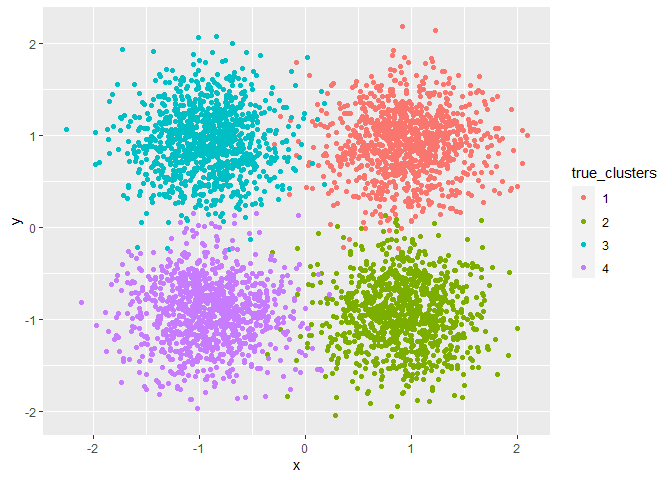
If our clustering works well, x and y should determine the partition while the other variables V1,..,V4 should be irrelevant. Feature importance is a novel way to determine whether this is the case. We’ll use the flexclust package for this example. Its main function FeatureImpCluster computes the permutation missclassification rate for each variable of the data. The mean misclassification rate over all iterations is interpreted as variable importance. The permutation missclassification rate of a feature (column) is the number of wrong cluster assignments divided by the number of observations (rows) given a permutation of the feature.
library(FeatureImpCluster)
library(flexclust)
#> Loading required package: grid
#> Loading required package: lattice
#> Loading required package: modeltools
#> Loading required package: stats4
set.seed(10)
res <- kcca(dat$data,k=4)
set.seed(10)
FeatureImp_res <- FeatureImpCluster(res,as.data.table(dat$data))
plot(FeatureImp_res)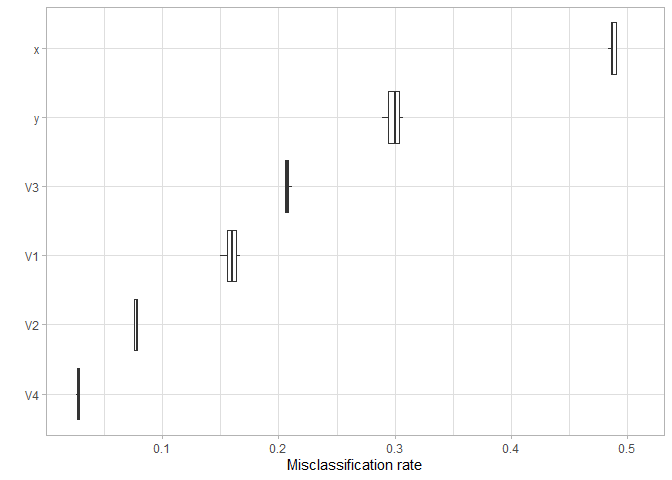
Indeed, y and x are most relevant. But also V3 has some impact on the cluster assignment. By looking at the cluster centers we see that, in particular, cluster 1 and 4 have a different center in the V3 dimension than the other clusters.
barplot(res)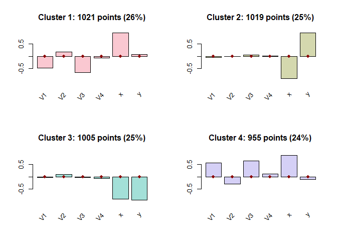
# bwplot(res,dat$data), image(res,which=5:6) # alternative diagnostic plots of flexclustIf we had a lot more than 6 variables (and possibly more clusters), then the chart above might be hard to interpret. The feature importance plot instead provides an aggregate statistics per feature and is, as such, always easy to interpret, in particular since only the top x (say, 10 or 30) features can be considered to get a first impression.
We know that the clustering is impacted by the random initialization. Thus it is usually recommended to run the clustering alogrithm several times with different seeds. As a by-product, the feature importance will provide us a feature selection mechanism: instead of iterating over permutation, we can iterate over the different cluster runs (or both). This way there is a good chance that any spurious importance is identified as an outlier.
For our example we repeat the clustering and feature importance calculation 20 times:
set.seed(12)
nr_seeds <- 20
seeds_vec <- sample(1:1000,nr_seeds)

savedImp <- data.frame(matrix(0,nr_seeds,dim(dat$data)[2]))
count <- 1
for (s in seeds_vec) {
  set.seed(s)
  res <- kcca(dat$data,k=4)
  set.seed(s)
  FeatureImp_res <- FeatureImpCluster(res,as.data.table(dat$data),sub = 1,biter = 1)
  savedImp[count,] <- FeatureImp_res$featureImp[sort(names(FeatureImp_res$featureImp))]
  count <- count + 1
}
names(savedImp) <- sort(names(FeatureImp_res$featureImp))
Now it becomes quite obvious that x and y are the only relevant features, and we could do our clustering only based on these features. This is important in practice since cluster centroids with a lower number of features are easier to interpret, and we can save time / money collecting and pre-processing unnecessary features.
boxplot(savedImp)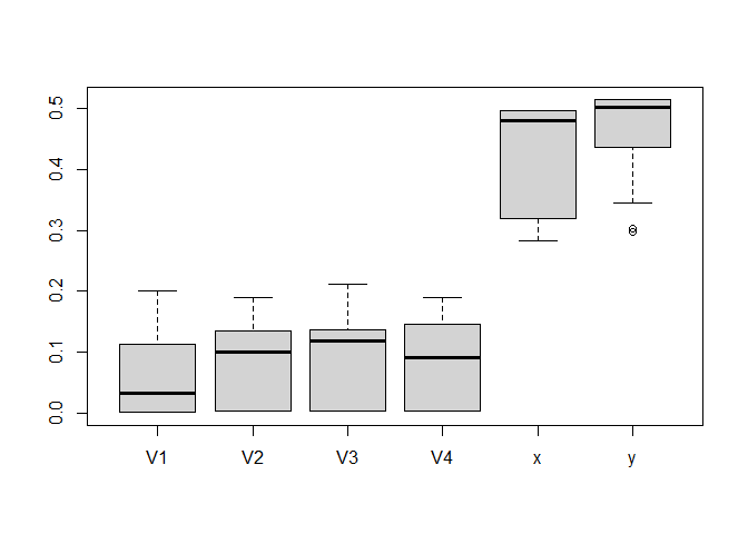
Another application arises for data sets with numerical and categorical features. Since one cannot simply calculate an Euclidean distance for categorical variables, one often uses an L0-norm (1 for equality, 0 else) for the latter and combines both metrics linearly with an appropriate weight (often this choice is referred to as Gower’s distance in the literature). In the clustMixType package the parameter lambda defines the trade off between Euclidean distance of numeric variables and simple matching coefficient between categorical variables. Feature Importance can be used as an additional guide to tune this parameter.
First we add categorical variables to our data set
ds <- as.data.table(dat$data)

n <- dim(ds)[1]
p <- dim(ds)[2]

set.seed(123)
ds[,cat1:=factor(rbinom(n,size=1,prob=0.3),labels = c("yes","no"))] # irrelevant factor
ds[,cat2:=factor(c(rep("yes",n/2),rep("no",n/2)))] # relevant factor
Obviously x and cat2 are strongly correlated.
cor(ds$x,as.numeric(ds$cat2),method="spearman")
#> [1] 0.8655712
First we’ll apply the clustering with an automatic estimation of lambda
library(clustMixType)
set.seed(123)
res <- kproto(x=ds,k=4)
#> # NAs in variables:
#>   V1   V2   V3   V4    x    y cat1 cat2
#>    0    0    0    0    0    0    0    0
#> 0 observation(s) with NAs.
#>
#> Estimated lambda: 2.17156
res$lambda
#> [1] 2.17156
With color=“type” we can draw the attention to the importance by data type. While cat2 correctly has some importance, the one of cat1 is almost zero.
set.seed(123)
FeatureImp_res <- FeatureImpCluster(res,ds)
plot(FeatureImp_res,ds,color="type")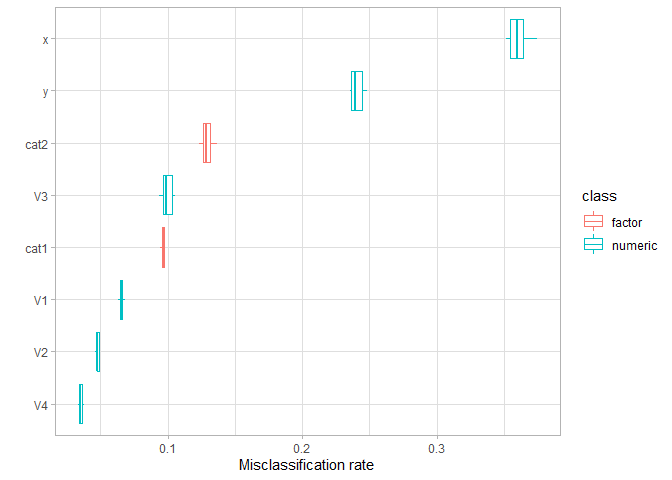
All in all the numeric variables are more important for the partitioning. If, for some reason, we wanted partitions that emphasize differences between the categorical features, we’d have to increase lambda. The feature importance directly shows us the effect of this action: the two categorical features now have an equally high importance a bit smaller than x but much higher than y.
set.seed(123)
res2 <- kproto(x=ds,k=4,lambda=3)
#> # NAs in variables:
#>   V1   V2   V3   V4    x    y cat1 cat2
#>    0    0    0    0    0    0    0    0
#> 0 observation(s) with NAs.
set.seed(123)
plot(FeatureImpCluster(res2,ds),ds,color="type")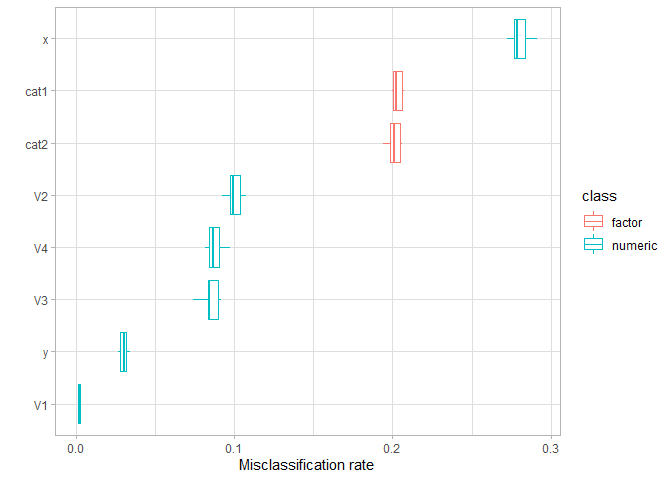
As above, repeated partitioning could be used to compute a more reasonable importance for the data set and not only an importance for a specific partition. Of course, further criteria should be used to determine an “optimal” lambda for the use case at hand - but certainly feature importance provides helpful guidance for data of mixed types.
FeatureImpCluster can be easily used with other packages. For example, stats::kmeans or cluster::pam can be used via flexclust:
cl_kcca <- flexclust::as.kcca(cl, dat$data) # cl is a kcca or pam object
FeatureImpCluster(cl_kcca,as.data.table(dat$data))
ClustImpute, a package that efficiently imputes missing values while performing a k-means clustering can be used directly:
library(ClustImpute)
res_clustimpute <- ClustImpute(as.data.frame(dat$data),4)

FeatureImpCluster(res_clustimpute,as.data.table(dat$data))
For other methods, a custom prediction function can be provided (cf. documentation for details)
FeatureImpCluster(clusterObj, data, predFUN = custom_prediction_function_for_clusterObj)There are further options not being explained in the examples above: