![]()
![]()
Table of contents: Overview - Installation - Usage - File types - Contact
RaMS is a lightweight package that provides rapid and
tidy access to mass-spectrometry data. This package is
lightweight because it’s built from the ground up rather than
relying on an extensive network of external libraries. No Rcpp, no
Bioconductor, no long load times and strange startup warnings. Just XML
parsing provided by xml2 and data handling provided by
data.table. Access is rapid because an absolute
minimum of data processing occurs. Unlike other packages,
RaMS makes no assumptions about what you’d like to do with
the data and is simply providing access to the encoded information in an
intuitive and R-friendly way. Finally, the access is tidy in
the philosophy of tidy
data. Tidy data neatly resolves the ragged arrays that mass
spectrometers produce and plays nicely with other tidy data packages.

To install the stable version on CRAN:
install.packages('RaMS')To install the current development version:
devtools::install_github("wkumler/RaMS", build_vignettes = TRUE)Finally, load RaMS like every other package:
library(RaMS)There’s only one main function in RaMS: the aptly named
grabMSdata. This function accepts the names of
mass-spectrometry files as well as the data you’d like to extract
(e.g. MS1, MS2, BPC, etc.) and produces a list of data tables. Each
table is intuitively named within the list and formatted tidily:
msdata_dir <- system.file("extdata", package = "RaMS")
msdata_files <- list.files(msdata_dir, pattern = "mzML", full.names=TRUE)

msdata <- grabMSdata(files = msdata_files[2:4], grab_what = c("BPC", "MS1"))
Some additional examples can be found below, but a more thorough
introduction can be found in the
vignette or by typing
vignette("Intro-to-RaMS", package = "RaMS") in the R
console after installation.
Base peak chromatograms (BPCs) and total ion chromatograms (TICs) have three columns, making them super-simple to plot with either base R or the popular ggplot2 library:
knitr::kable(head(msdata$BPC, 3))| rt | int | filename |
|---|---|---|
| 4.009000 | 11141859 | LB12HL_AB.mzML.gz |
| 4.024533 | 9982309 | LB12HL_AB.mzML.gz |
| 4.040133 | 10653922 | LB12HL_AB.mzML.gz |
plot(msdata$BPC$rt, msdata$BPC$int, type = "l", ylab="Intensity")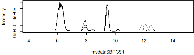
library(ggplot2)
ggplot(msdata$BPC) + geom_line(aes(x = rt, y=int, color=filename)) +
  facet_wrap(~filename, scales = "free_y", ncol = 1) +
  labs(x="Retention time (min)", y="Intensity", color="File name: ") +
  theme(legend.position="top")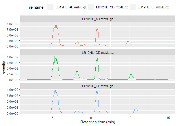
MS1 data includes an additional dimension, the m/z of each ion measured, and has multiple entries per retention time:
knitr::kable(head(msdata$MS1, 3))| rt | mz | int | filename |
|---|---|---|---|
| 4.009 | 139.0503 | 1800550.12 | LB12HL_AB.mzML.gz |
| 4.009 | 148.0967 | 206310.81 | LB12HL_AB.mzML.gz |
| 4.009 | 136.0618 | 71907.15 | LB12HL_AB.mzML.gz |
This tidy format means that it plays nicely with other tidy data
packages. Here, we use data.table and
a few other tidyverse packages to compare a molecule’s 13C
and 15N peak areas to that of the base peak, giving us some
clue as to its molecular formula. Note also the use of the
trapz function (available in v1.3.2+) to calculate the area
of the peak given the retention time and intensity values.
library(data.table)
library(tidyverse)

M <- 118.0865
M_13C <- M + 1.003355
M_15N <- M + 0.997035

iso_data <- imap_dfr(lst(M, M_13C, M_15N), function(mass, isotope){
  peak_data <- msdata$MS1[mz%between%pmppm(mass) & rt%between%c(7.6, 8.2)]
  cbind(peak_data, isotope)
})

iso_data %>%
  group_by(filename, isotope) %>%
  summarise(area=trapz(rt, int)) %>%
  pivot_wider(names_from = isotope, values_from = area) %>%
  mutate(ratio_13C_12C = M_13C/M) %>%
  mutate(ratio_15N_14N = M_15N/M) %>%
  select(filename, contains("ratio")) %>%
  pivot_longer(cols = contains("ratio"), names_to = "isotope") %>%
  group_by(isotope) %>%
  summarize(avg_ratio = mean(value), sd_ratio = sd(value), .groups="drop") %>%
  mutate(isotope=str_extract(isotope, "(?<=_).*(?=_)")) %>%
knitr::kable()| isotope | avg_ratio | sd_ratio |
|---|---|---|
| 13C | 0.0544072 | 0.0005925 |
| 15N | 0.0033611 | 0.0001578 |
With natural abundances for 13C and 15N of 1.11% and 0.36%, respectively, we can conclude that this molecule likely has five carbons and a single nitrogen.
Of course, it’s always a good idea to plot the peaks and perform a manual check of data quality:
ggplot(iso_data) +
  geom_line(aes(x=rt, y=int, color=filename)) +
  facet_wrap(~isotope, scales = "free_y", ncol = 1)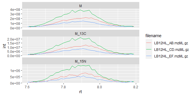
MS1 data typically consists of many individual chromatograms, so RaMS provides a small function that can bin it into chromatograms based on m/z windows.
msdata$MS1 %>%
  arrange(desc(int)) %>%
  mutate(mz_group=mz_group(mz, ppm=10, max_groups = 3)) %>%
  qplotMS1data(facet_col = "mz_group")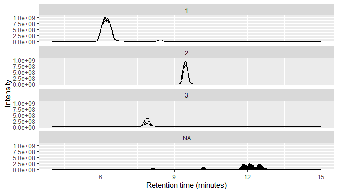
We also use the qplotMS1data function above, which wraps
the typical ggplot call to avoid needing to type out
ggplot() + geom_line(aes(x=rt, y=int, group=filename))
every time. Both the mz_group and qplotMS1data
functions were added in RaMS version 1.3.2.
DDA (fragmentation) data can also be extracted, allowing rapid and intuitive searches for fragments or neutral losses:
msdata <- grabMSdata(files = msdata_files[1], grab_what = "MS2")For example, we may be interested in the major fragments of a specific molecule:
msdata$MS2[premz%between%pmppm(351.0817) & int>mean(int)] %>%
  plot(int~fragmz, type="h", data=., ylab="Intensity", xlab="Fragment m/z")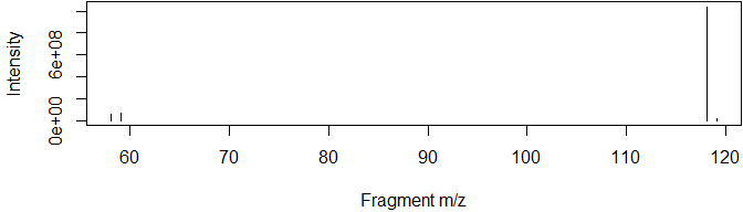
Or want to search for precursors with a specific neutral loss above a certain intensity:
msdata$MS2[, neutral_loss:=premz-fragmz][int>1e4] %>%
  filter(neutral_loss%between%pmppm(126.1408, 5)) %>%
head(3) %>% knitr::kable()| rt | premz | fragmz | int | voltage | filename | neutral_loss |
|---|---|---|---|---|---|---|
| 47.27750 | 351.0817 | 224.9409 | 16333.23 | 40 | Blank_129I_1L_pos_20240207-MS3.mzML.gz | 126.1408 |
| 47.35267 | 351.0818 | 224.9410 | 27353.09 | 40 | Blank_129I_1L_pos_20240207-MS3.mzML.gz | 126.1408 |
| 47.42767 | 351.0818 | 224.9410 | 33843.92 | 40 | Blank_129I_1L_pos_20240207-MS3.mzML.gz | 126.1408 |
Selected/multiple reaction monitoring files don’t have data stored in
the typical MSn format but instead encode their values as chromatograms.
To extract data in this format, include "chroms" in the
grab_what argument:
chromsdata <- grabMSdata(files = msdata_files[7], grab_what = "chroms", verbosity = 0)which has individual reactions separated by the
chrom_type column (and the associated index) with relevant
target/fragment data:
knitr::kable(head(chromsdata$chroms, 3))| chrom_type | chrom_index | target_mz | product_mz | rt | int | filename |
|---|---|---|---|---|---|---|
| TIC | 0 | NA | NA | 2.000000 | 0 | wk_chrom.mzML.gz |
| TIC | 0 | NA | NA | 2.048077 | 0 | wk_chrom.mzML.gz |
| TIC | 0 | NA | NA | 2.096154 | 0 | wk_chrom.mzML.gz |
As of version 1.1.0, RaMS has functions that allow
irrelevant data to be removed from the file to reduce file sizes. See
the vignette
for more details.
Version 1.2.0 of RaMS introduced a new file type, the “transposed mzML” or “tmzML” file to resolve the large memory requirement when working with many files. See the vignette for more details, though note that I’ve largely deprecated this file type in favor of proper database solutions as in the speed & size comparison vignette.
RaMS is currently limited to the modern mzML data
format and the slightly older mzXML format. Tools to
convert data from other formats are available through Proteowizard’s
msconvert tool. Data can, however, be gzip compressed (file
ending .gz) and this compression actually speeds up data retrieval
significantly as well as reducing file sizes.
Currently, RaMS handles MS1, MS2,
and MS3 data. This should be easy enough to expand in the
future, but right now I haven’t observed a demonstrated need for higher
fragmentation level data collection.
Additionally, note that files can be streamed from the internet
directly if a URL is provided to grabMSdata, although this
will usually take longer than reading a file from disk:
## Not run:
# Find a file with a web browser:
browseURL("https://www.ebi.ac.uk/metabolights/MTBLS703/files")

# Copy link address by right-clicking "download" button:
sample_url <- paste0("https://www.ebi.ac.uk/metabolights/ws/studies/MTBLS703/",
                     "download/acefcd61-a634-4f35-9c3c-c572ade5acf3?file=",
                     "FILES/161024_Smp_LB12HL_AB_pos.mzXML")

msdata <- grabMSdata(sample_url, grab_what="everything", verbosity=2)
msdata$metadata
For an analysis of how RaMS compares to other methods of MS data access and alternative file types, consider browsing the speed & size comparison vignette.
Feel free to submit questions, bugs, or feature requests on the GitHub Issues page.
README last built on 2024-09-19