
The ShellChron package contains all formulae and documentation required to run the ShellChron model. The ShellChron model uses stable oxygen isotope records (d18O) from seasonal paleo-archives to create an age model for the archive.
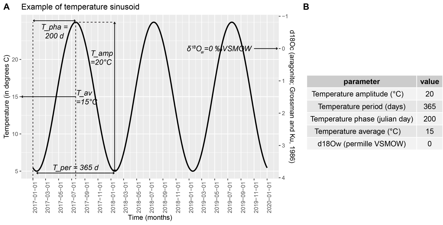
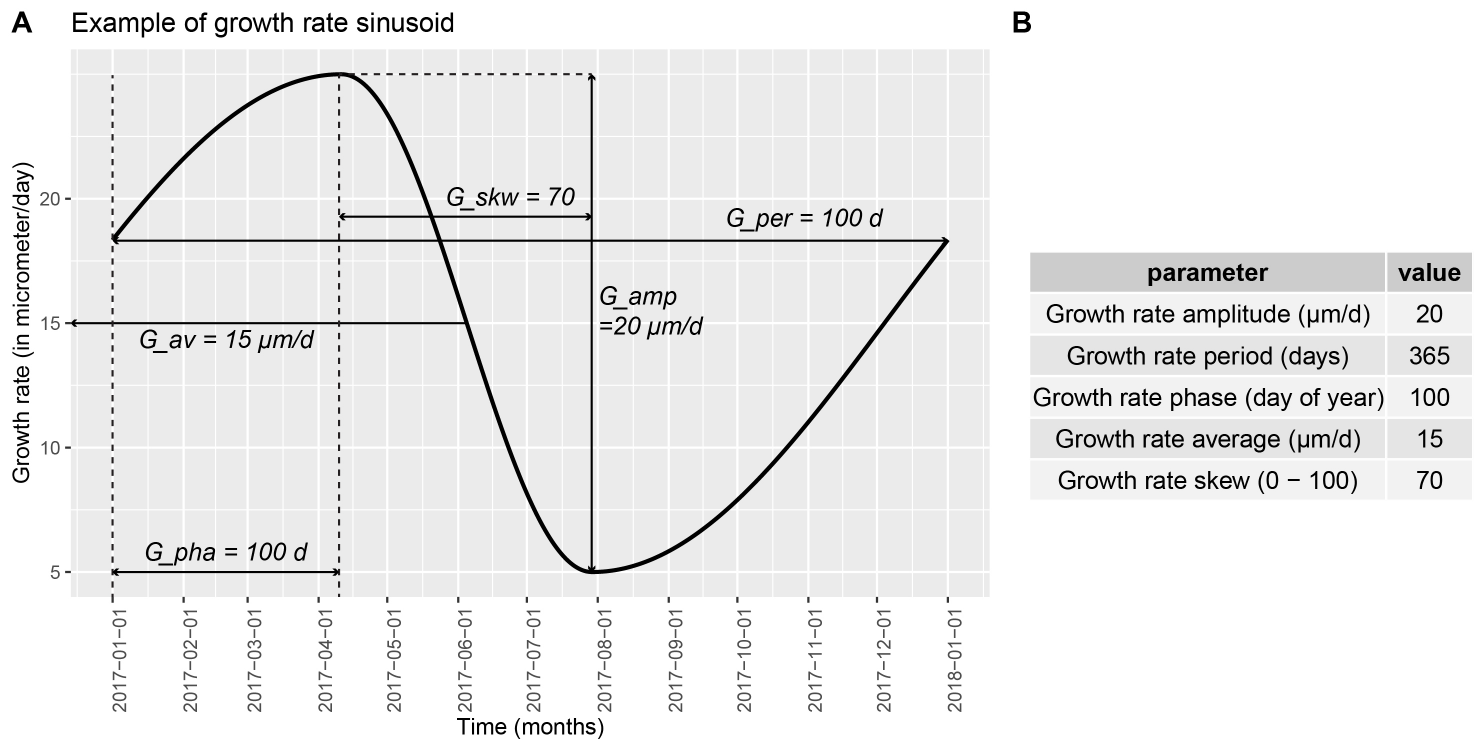
In short, ShellChron feeds a temperature sinusoid (Figure 1; see details in “temperature_curve()” function) and a skewed growth rate sinusoid (Figure 2; see details in “growth_rate_curve()” function) to a d18O model (see details in “d18O_model()” function). The resulting modeled d18O is then compared with the user-provided d18O data and the parameters of the temperature and growth rate functions are optimized using the SCEUA algorithm (see Duan et al., 1992) to match the d18O data. As a result, the timing of each data point with reference to the seasonal cycle is exported, from which an age model for the entire record can be constructed.
The model builds on previous work by Judd et al. 2018 and expands on this previous model in several key ways:
NOTE: To run optimally, ShellChron requires sampling distance data to be provided in micrometers (see “data_import()” function). The optimal structure of the input CSV should be as follows (see description in “Virtual_shell” example):
column 1: D Sampling distance, in micrometers along the virtual record.
column 2: d18Oc stable oxygen isotope value, in permille VPDB.
column 3: YEARMARKER Vector of zeroes with “1” marking year transitions.
column 4: D_err Sampling distance uncertainty, in micrometers.
column 5: d18Oc_err stable oxygen isotope value uncertainty, in permille.
You can install the released version of ShellChron from CRAN with:
install.packages("ShellChron")And the development version from GitHub with:
# install.packages("devtools")
devtools::install_github("nielsjdewinter/ShellChron")This is a basic example which shows you how to solve a common problem:
library(ShellChron)
## Full model run
# WARNING: Running the full ShellChron model (even on small example data) always takes some time (usually in the order of 30-60 minutes)
# example <- wrap_function(path = getwd(),
#  file_name = system.file("extdata", "Virtual_shell.csv",
#  package = "ShellChron"),
#  "calcite",
#  1,
#  365,
#  d18Ow = 0,
#  t_maxtemp = 182.5,
#  MC = 1000,
#  plot = FALSE,
#  plot_export = FALSE,
#  export_raw = FALSE)"

# Quick demo on how to create an SST curve
# Set parameters
T_amp <- 20
T_per <- 365
T_pha <- 150
T_av <- 15
T_par <- c(T_amp, T_per, T_pha, T_av)
SST <- temperature_curve(T_par, 1, 1) # Run the function