This package introduces:
wideplot() graphics for exploring the structure of a
dataset through a grid of variables and graphic types.longplot() graphics, which present the entire catalog
of available graphics for representing one particular variable or a
limited selection of variables using a grid of graphic types and
variations on these types.matrixplot() graphics, a generalization of a pairs plot
in the sense that the graphic that is replicated in each cell of the
matrix can be selected from the catalogue of bivariate graphics.plotup() function, which complements the previous three
functions in that it presents a particular graphic for a specific
variable or a limited number of variables of a dataset.Future work will include the ability to draw longplot()
and plotup() graphics from a selection of a wider number
and combinations of types of variables within a dataset.
You can install the released version of brinton from CRAN with:
install.packages("brinton")And then load the functions included in the package:
library(brinton)
#> Warning: replacing previous import 'lifecycle::last_warnings' by
#> 'rlang::last_warnings' when loading 'tibble'
#> Warning: replacing previous import 'lifecycle::last_warnings' by
#> 'rlang::last_warnings' when loading 'pillar'
#> M a G i C i N G R a P H SWhen a new dataset comes up, R users use to call the
str() function that describes textually the main
characteristics of this dataset. The new wideplot()
function does the same but graphically. As an example, just run:
wideplot(esoph)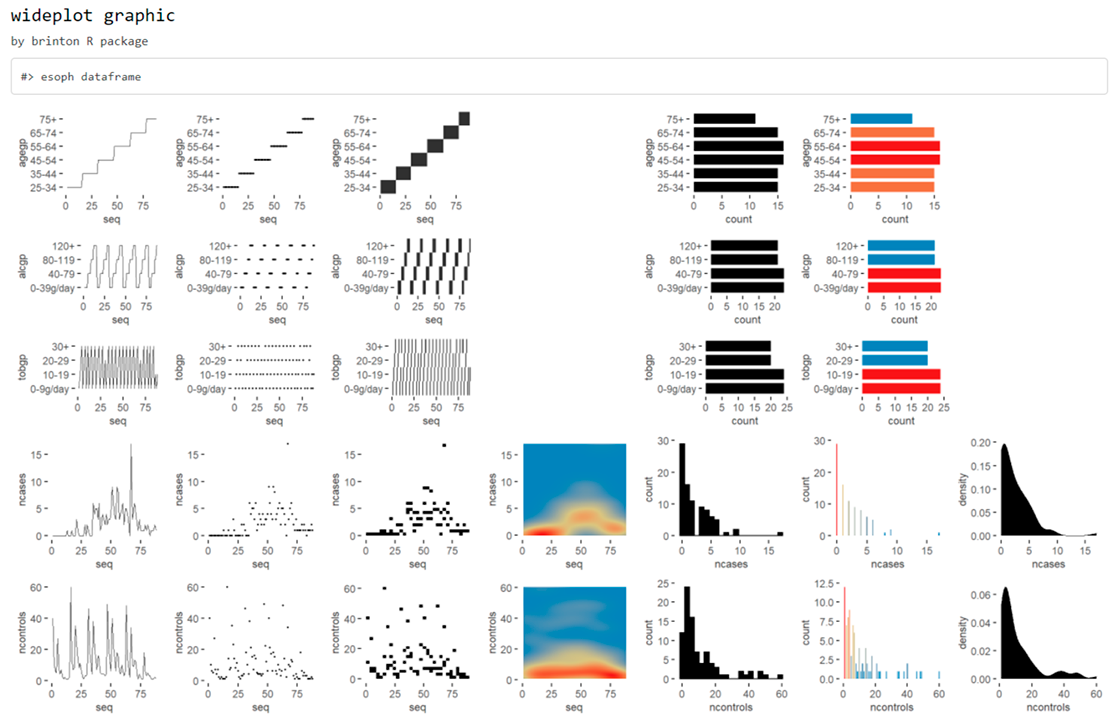
This function includes the argument dataclass that sets
the types of variables to be included in the grid as well as the order
in which they are listed. As an example, the following line will plot
only the numeric variables included in the iris dataset:
wideplot(esoph, dataclass = c("numeric"))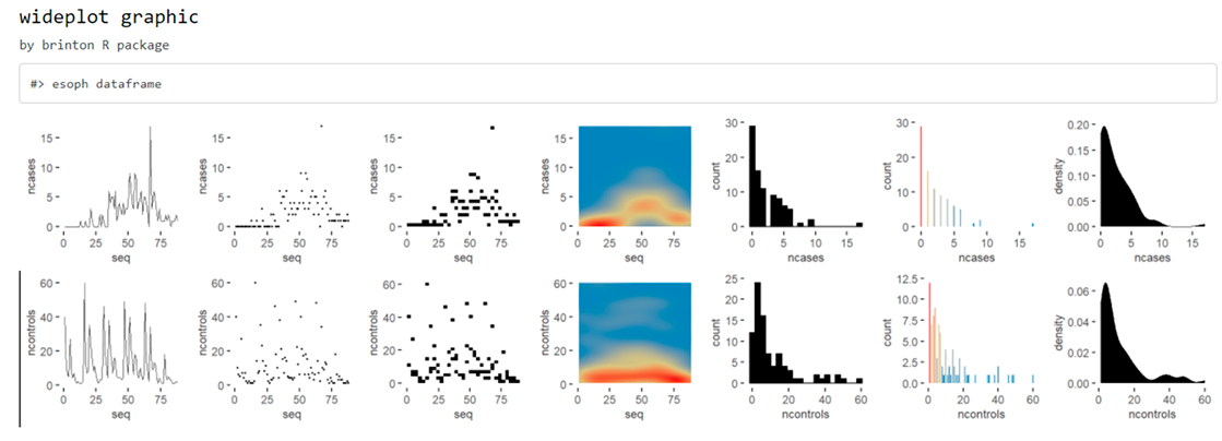
Although, the wideplot() function shows only a small set
of the graphics suitable for each type of data. If the user wants to see
all the available graphics for some specific variable or a combination
of two specific variables included in the dataset, then the
longplot() is useful. As an example, just run:
longplot(esoph, "alcgp")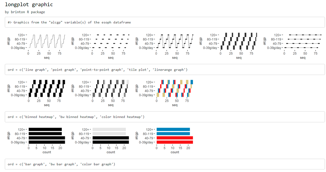
longplot(esoph, c("alcgp", "agegp"))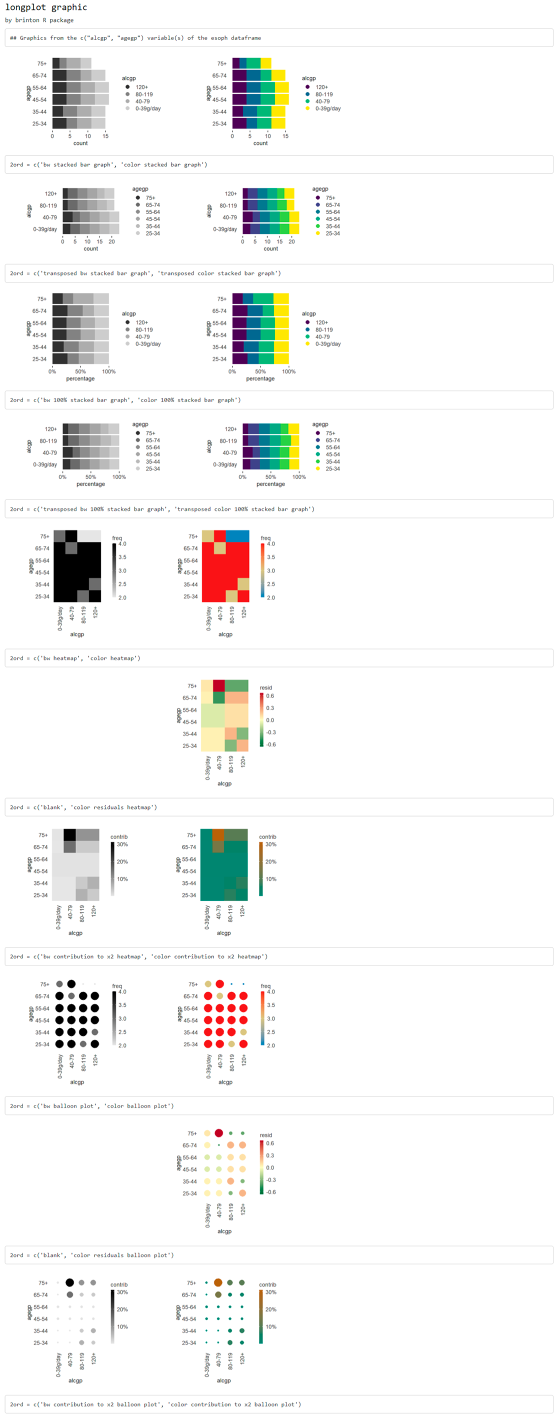
Any of the graphics presented in the longplot() output
can also be included as an output of the wideplot()
function. If one wants to compare the output of some other specific
graphics one can, for instance, run:
wideplot(
  esoph,
  dataclass = c("numeric"),
  numeric = c("point graph", "binned heatmap", "bw binned heatmap", "color binned heatmap"),
  label = TRUE
)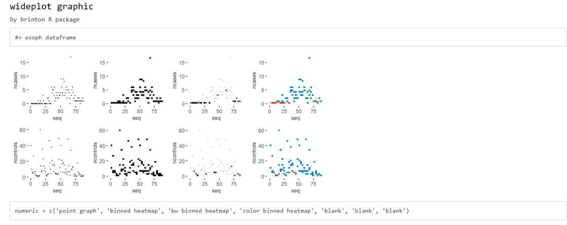
Sometimes, specially with character variables, there is not enought
space for the graphic area, and the user may want to increase the width
of the columns in the matrix. The user can then modify the defalut value
of the ncol argument:
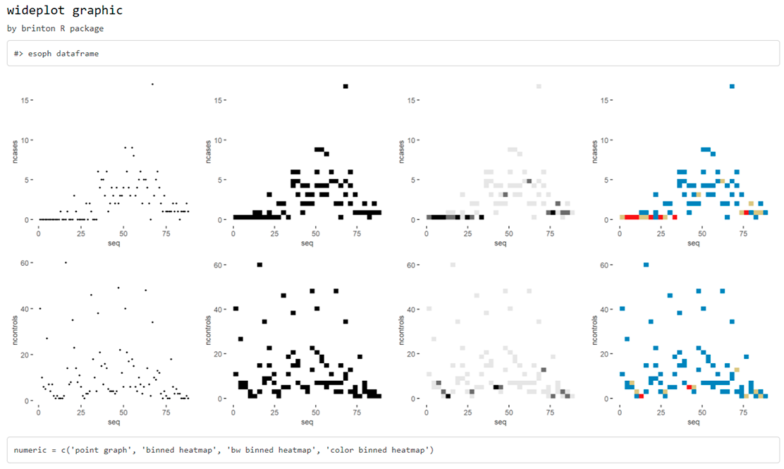
wideplot(
  esoph,
  dataclass = c("numeric"),
  numeric = c("point graph", "binned heatmap", "bw binned heatmap", "color binned heatmap"),
  label = TRUE,
  ncol = 4
)
While the wideplot function displays a grid of univariate graphics, if a matrix of bivariate graphics is intended for variables of one particular type, the matrixplot() function is useful. Type for instance the following code:
matrixplot(esoph, dataclass = "ordered", diagram = "color heatmap")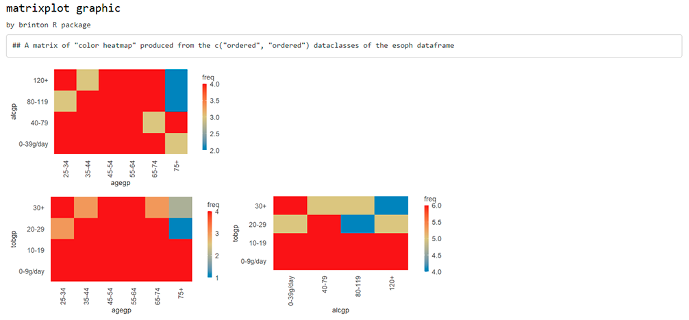
Same thing if the desired matrix has to include graphics from variables of two different types (please note that the graphic type has to be compatible):
matrixplot(esoph, dataclass = c("numeric", "ordered"), diagram = "box plot")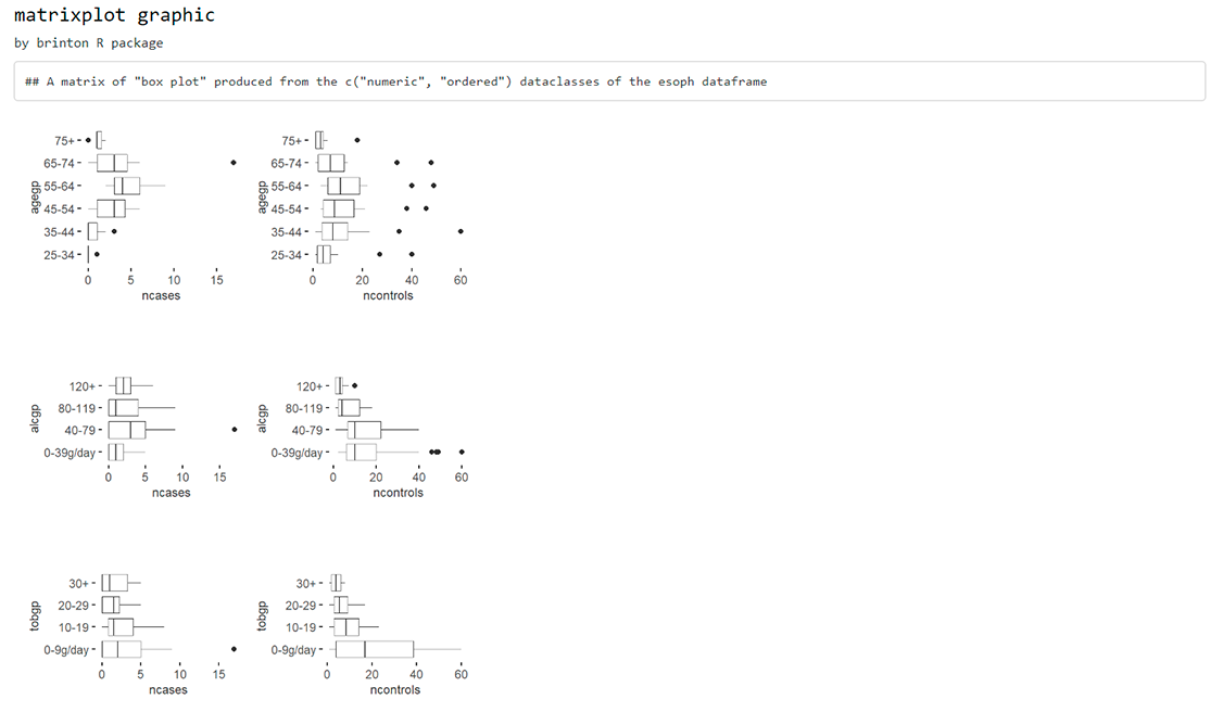
If the user is interested in one particular graphic then the function
plotup() is useful.
plotup(esoph, "ncases", "color histogram")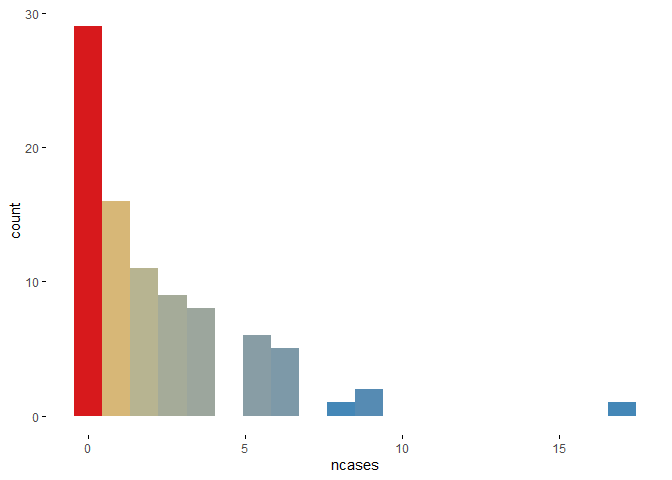
Or, as an example of a graphic that requires more than one input variable:
plotup(esoph, c("agegp", "alcgp"), "color stacked bar graph")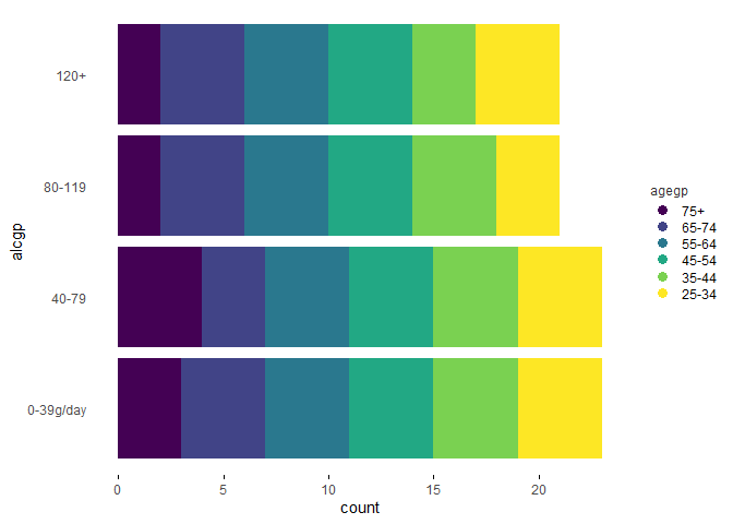
The default output of the plotup() function is a
c("gg", "ggplot") object but the output
argument allows, as a side effect, to write and present the graphic in a
html file or to print the ggplot2 function in the console:
plotup(esoph, c("agegp", "alcgp"), "color stacked bar graph", output = "html")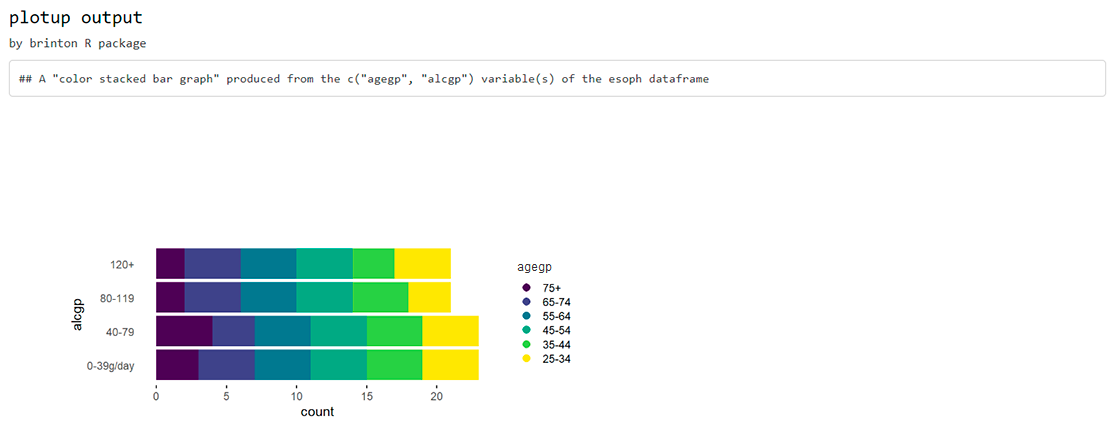
plotup(esoph, c("agegp", "alcgp"), "color stacked bar graph", output = "console")
#>
#> ggplot(esoph, aes(x=alcgp, fill=agegp)) +
#>   geom_bar(key_glyph = draw_key_dotplot, position = 'stack') +
#>   viridis::scale_fill_viridis(discrete=TRUE, direction = -1) +
#>   guides(fill=guide_legend(title='agegp',
#>     keyheight = unit(0.4, 'cm'),
#>     title.theme = element_text(size = 9, colour = 'gray20'),
#>     reverse = TRUE)) +
#>   coord_flip() +
#>   theme_minimal() +
#>   theme(panel.grid = element_line(colour = NA),
#>     axis.ticks.x = element_line(color = 'black'))