![]()
![]()
![]()
Accelerate computational Bayesian inference workflows in R
through interactive modelling, visualization, and inference. The package
leverages directed acyclic graphs (DAGs) to create a unified language
language for business stakeholders, statisticians, and programmers. Due
to its visual nature and simple model construction, causact
serves as a great entry-point for newcomers to computational Bayesian
inference.
The
causactpackage offers robust support for both foundational and advanced Bayesian models. While introductory models are well-covered, the utilization of multi-variate distributions such as multi-variate normal, multi-nomial, or dirichlet distributions, may not work as expected. There are ongoing enhancements in the pipeline to facilitate construction of these more intricate models.
While proficiency in R is the only requirement for users of this
package, it also functions as a introductory probabilistic programming
language, seamlessly incorporating the numpyro Python
package to facilitate Bayesian inference without the need to learn any
syntax outside of the package or R. Furthermore, the package streamlines
the process of indexing categorical variables, which often presents a
complex syntax hurdle for those new to computational Bayesian
methods.
For enhanced learning, the causact package for Bayesian
inference is featured in
A Business Analyst's Introduction to Business Analytics
available at https://www.causact.com/.
Feedback and encouragement is appreciated via github issues.
To install the causact package, follow the steps
outlined below:
For the current stable release, which is tailored to integrate with
Python’s numpyro package, employ the following command:
install.packages("causact")Then, see Essential
Dependencies if you want to be able to automate sampling using the
numpyro package.
If you want the most recent development version (not recommended), execute the following:
install.packages("remotes")
remotes::install_github("flyaflya/causact")To harness the full potential of causact for DAG
visualization and Bayesian posterior analysis, it’s vital to ensure
proper integration with the numpyro package. Given the
Python-based nature of numpyro, a few essential
dependencies must be in place. Execute the following commands after
installing causact:
library(causact)
install_causact_deps()
If prompted, respond with Y to any inquiries related to
installing miniconda.
Note: If opting for installation on Posit Cloud, temporarily adjust your project’s RAM to 4GB during the installation process (remember to APPLY CHANGES). This preemptive measure helps avoid encountering an
Error: Error creating conda environment [exit code 137]. After installation, feel free to revert the settings to 1GB of RAM.
Note: The September 11, 2023 release of
reticulate(v1.32) has caused an issue which gives aTypeError: the first argument must be callableerror when usingdag_numpyro()on windows. If you experience this, install the dev version ofreticulateby following the below steps:
Install RTOOLS by using installer at: https://cran.r-project.org/bin/windows/Rtools/
Run this to get the dev version of
reticulate:
# install DEV version of reticulate
# install.packages("pak") #uncomment as needed
pak::pak("rstudio/reticulate")In cases where legacy compatibility is paramount and you still rely
on the operationality of the dag_greta() function, consider
installing v0.4.2 of the causact package.
However, it’s essential to emphasize that this approach is not
recommended for general usage:
### EXERCISE CAUTION BEFORE EXECUTING THESE LINES
### Only proceed if dag_greta() is integral to your existing codebase
install.packages("remotes")
remotes::install_github("flyaflya/causact@v0.4.2")
Your judicious choice of installation method will ensure a seamless
and effective integration of the causact package into your
computational toolkit.
Example taken from https://www.causact.com/graphical-models-tell-joint-distribution-stories.html#graphical-models-tell-joint-distribution-stories
with the packages dag_foo() functions further described
here:
#> Initializing python, numpyro, and other dependencies. This may take up to 15 seconds...
#> Initializing python, numpyro, and other dependencies. This may take up to 15 seconds...COMPLETED!
#>
#> Attaching package: 'causact'
#> The following objects are masked from 'package:stats':
#>
#>     binomial, poisson
#> The following objects are masked from 'package:base':
#>
#> beta, gammalibrary(causact)
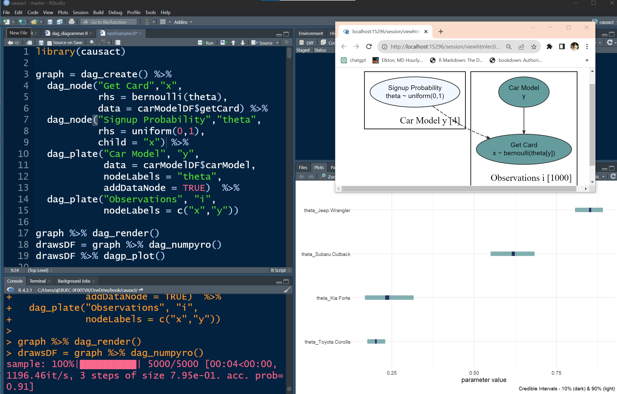
graph = dag_create() %>%
dag_node(descr = "Get Card", label = "y",
rhs = bernoulli(theta),
data = carModelDF$getCard) %>%
dag_node(descr = "Card Probability", label = "theta",
rhs = beta(2,2),
child = "y") %>%
dag_plate(descr = "Car Model", label = "x",
data = carModelDF$carModel,
nodeLabels = "theta",
addDataNode = TRUE)
graph %>% dag_render()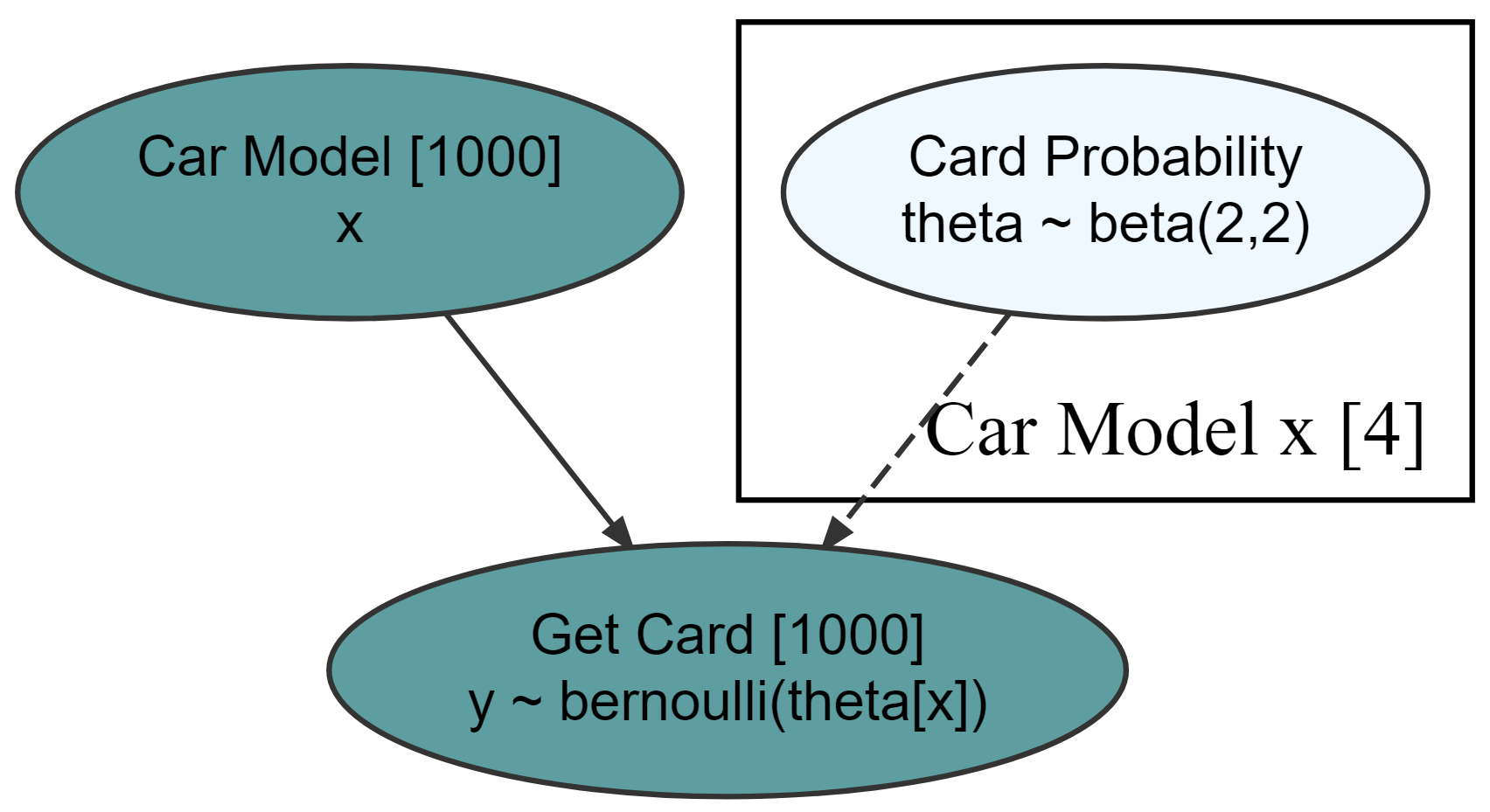
graph %>% dag_render(shortLabel = TRUE)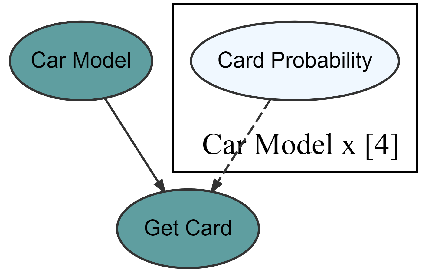
numpyro codedrawsDF = graph %>% dag_numpyro()
drawsDF ### see top of data frame
#> # A tibble: 4,000 × 4
#> theta_Toyota.Corolla theta_Subaru.Outback theta_Kia.Forte theta_Jeep.Wrangler
#> <dbl> <dbl> <dbl> <dbl>
#> 1 0.215 0.582 0.226 0.839
#> 2 0.194 0.643 0.264 0.853
#> 3 0.216 0.602 0.243 0.831
#> 4 0.217 0.647 0.177 0.843
#> 5 0.186 0.580 0.309 0.853
#> 6 0.230 0.633 0.237 0.846
#> 7 0.217 0.619 0.263 0.859
#> 8 0.205 0.692 0.274 0.862
#> 9 0.191 0.693 0.332 0.847
#> 10 0.188 0.655 0.174 0.851
#> # ℹ 3,990 more rowsNote: if you have used older versions of causact, please know that dag_numpyro() is a drop-in replacement for dag_greta().
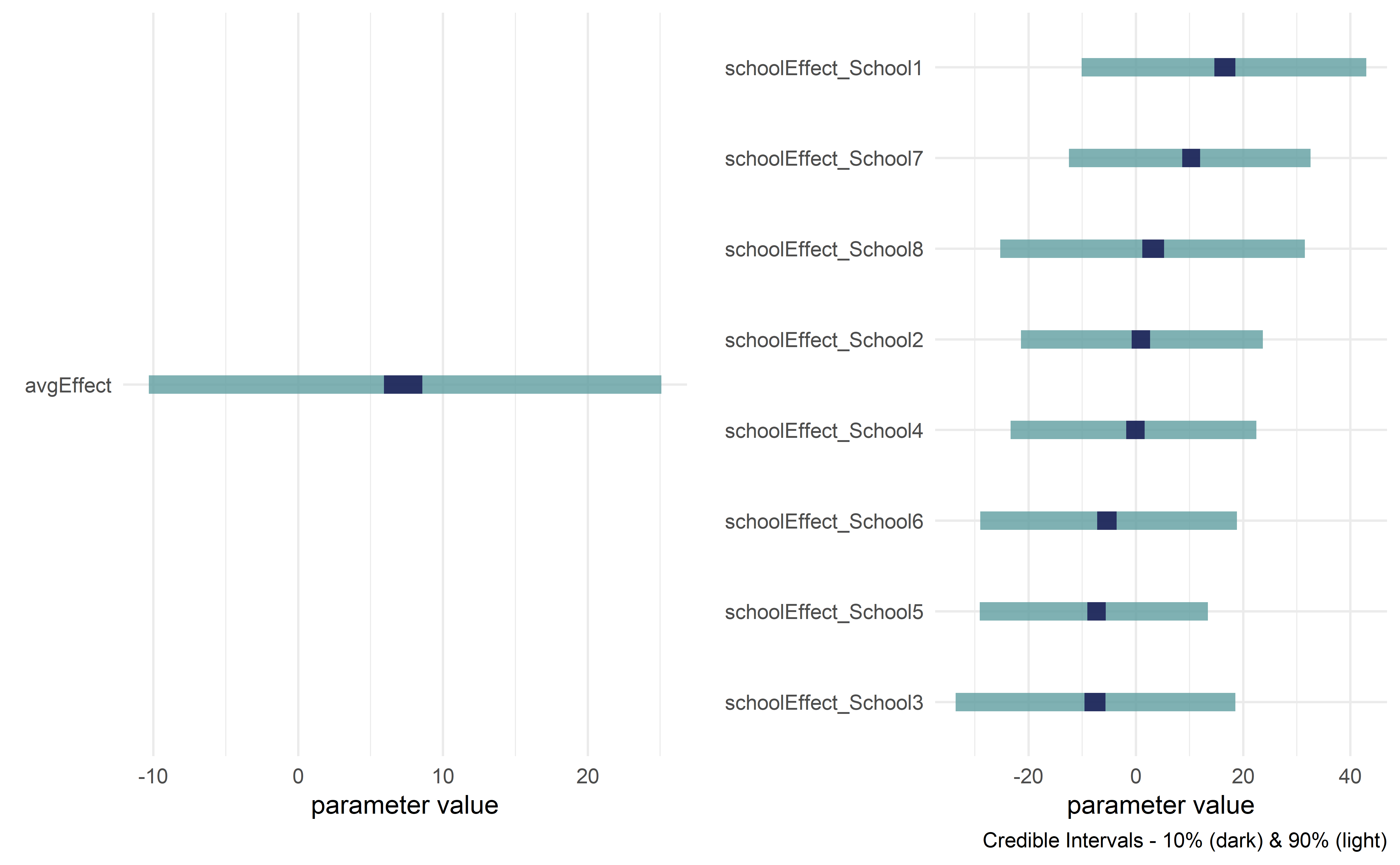
drawsDF %>% dagp_plot()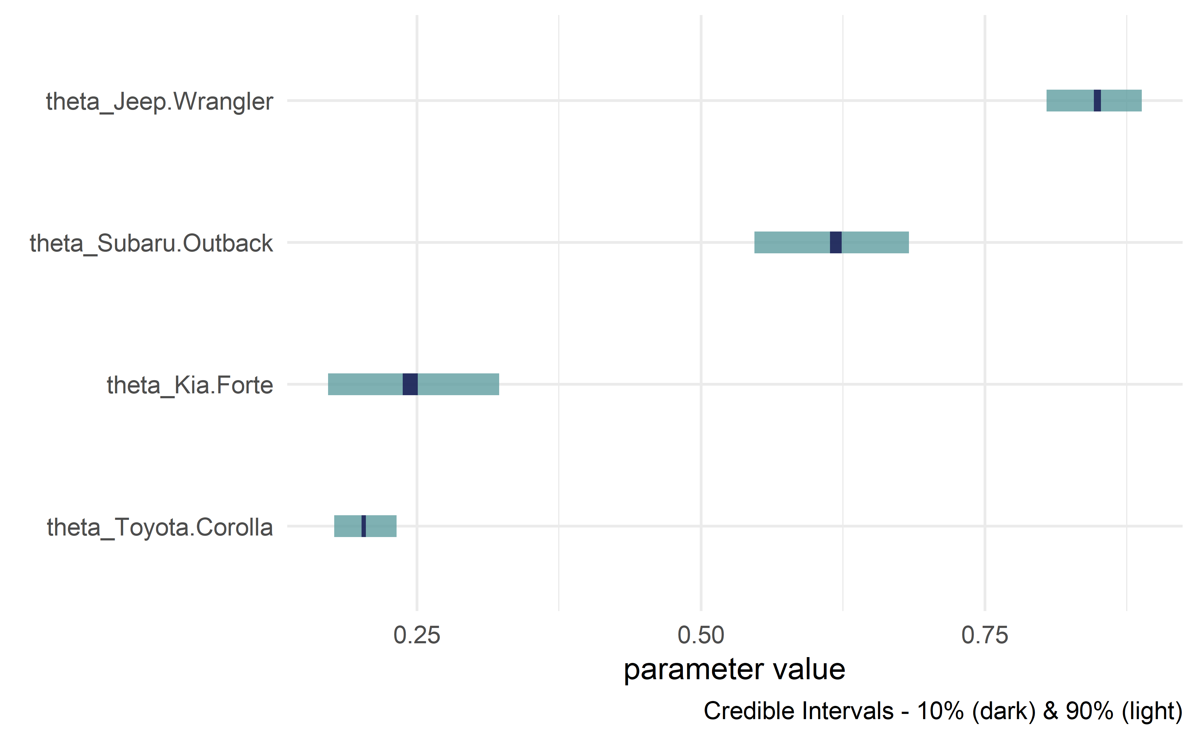
Credible interval plots.
numpyro code without executing it (for debugging or
learning)numpyroCode = graph %>% dag_numpyro(mcmc = FALSE)
#>
#> ## The below code will return a posterior distribution
#> ## for the given DAG. Use dag_numpyro(mcmc=TRUE) to return a
#> ## data frame of the posterior distribution:
#> reticulate::py_run_string("
#> import numpy as np
#> import numpyro as npo
#> import numpyro.distributions as dist
#> import pandas as pd
#> from jax import random
#> from numpyro.infer import MCMC, NUTS
#> from jax.numpy import transpose as t
#> from jax.numpy import (exp, log, log1p, expm1, abs, mean,
#> sqrt, sign, round, concatenate, atleast_1d,
#> cos, sin, tan, cosh, sinh, tanh,
#> sum, prod, min, max, cumsum, cumprod )
#> ## note that above is from JAX numpy package, not numpy.
#>
#> y = np.array(r.carModelDF.getCard) #DATA
#> x = pd.factorize(np.array(r.carModelDF.carModel),use_na_sentinel=True)[0] #DIM
#> x_dim = len(np.unique(x)) #DIM
#> x_crd = pd.factorize(np.array(r.carModelDF.carModel),use_na_sentinel=True)[1] #DIM
#> def graph_model(y,x):
#> ## Define random variables and their relationships
#> with npo.plate('x_dim',x_dim):
#> theta = npo.sample('theta', dist.Beta(2,2))
#>
#> y = npo.sample('y', dist.Bernoulli(theta[x]),obs=y)
#>
#>
#> # computationally get posterior
#> mcmc = MCMC(NUTS(graph_model), num_warmup = 1000, num_samples = 4000)
#> rng_key = random.PRNGKey(seed = 1234567)
#> mcmc.run(rng_key,y,x)
#> axis_labels = {'x_dim': x_crd}
#> rv_to_axes = {'theta': ['x_dim']}
#> drop_names = set()
#> samples = mcmc.get_samples(group_by_chain=True) # dict: name -> [chains, draws, *axes]
#> import numpy as np, pandas as pd, string
#> # Flatten (chains*draws) and expand RVs using rv_to_axes + axis_labels
#> flat = {name: np.reshape(val, (-1,) + val.shape[2:]) for name, val in list(samples.items())}
#> out = {}
#> allowed = set(string.ascii_letters + string.digits + '._')
#> def sanitize_label(s):
#> s = str(s).strip().replace(' ', '.') # spaces -> dots
#> s = ''.join((ch if ch in allowed else '.') for ch in s)
#> # collapse repeated dots without regex
#> while '..' in s:
#> s = s.replace('..', '.')
#> s = s.strip('.')
#> return s if s else '1'
#>
#> for name, arr in list(flat.items()):
#> # Drop deterministic RVs entirely
#> if name in drop_names:
#> continue
#> axes = rv_to_axes.get(name, []) # [] if not present
#> # If scalar per draw, keep as a single column
#> if arr.ndim == 1:
#> out[name] = arr
#> continue
#> # Otherwise (vector/matrix/...): expand to separate columns
#> trailing = arr.shape[1:]
#> arr2 = arr.reshape(arr.shape[0], int(np.prod(trailing)))
#> for j in range(arr2.shape[1]):
#> idx = np.unravel_index(j, trailing)
#> parts = []
#> for axis, i in enumerate(idx):
#> if axis < len(axes):
#> axis_name = axes[axis]
#> labels = axis_labels.get(axis_name)
#> if labels is not None:
#> labs = np.asarray(labels).astype(str)
#> lab = labs[i] if i < labs.shape[0] else str(i + 1)
#> parts.append(sanitize_label(lab))
#> else:
#> parts.append(str(i + 1))
#> else:
#> parts.append(str(i + 1))
#> # No brackets; join labels with '_' so tibble won't append trailing dots
#> col = name if not parts else name + '_' + '_'.join(parts)
#> out[col] = arr2[:, j]
#> drawsDF = pd.DataFrame(out)"
#> ) ## END PYTHON STRING
#> drawsDF = reticulate::py$drawsDFWhether you encounter a clear bug, have a suggestion for improvement, or just have a question, we are thrilled to help you out. In all cases, please file a GitHub issue. If reporting a bug, please include a minimal reproducible example.
We welcome help turning causact into the most intuitive
and fastest method of converting stakeholder narratives about
data-generating processes into actionable insight from posterior
distributions. If you want to help us achieve this vision, we welcome
your contributions after reading the new
contributor guide. Please note that this project is released with a
Contributor
Code of Conduct. By participating in this project you agree to abide
by its terms.
For more info, see
A Business Analyst's Introduction to Business Analytics
available at https://www.causact.com. You can also check out the
package’s vignette:
vignette("narrative-to-insight-with-causact"). Two
additional examples are shown below.
McElreath, Richard. Statistical rethinking: A Bayesian course with examples in R and Stan. Chapman and Hall/CRC, 2018.
library(tidyverse)
library(causact)

# data object used below, chimpanzeesDF, is built-in to causact package

graph = dag_create() %>%
  dag_node("Pull Left Handle","L",
           rhs = bernoulli(p),
           data = causact::chimpanzeesDF$pulled_left) %>%
  dag_node("Probability of Pull", "p",
           rhs = 1 / (1 + exp(-((alpha + gamma + beta)))),
           child = "L") %>%
  dag_node("Actor Intercept","alpha",
           rhs = normal(alphaBar, sigma_alpha),
           child = "p") %>%
  dag_node("Block Intercept","gamma",
           rhs = normal(0,sigma_gamma),
           child = "p") %>%
  dag_node("Treatment Intercept","beta",
           rhs = normal(0,0.5),
           child = "p") %>%
  dag_node("Actor Population Intercept","alphaBar",
           rhs = normal(0,1.5),
           child = "alpha") %>%
  dag_node("Actor Variation","sigma_alpha",
           rhs = exponential(1),
           child = "alpha") %>%
  dag_node("Block Variation","sigma_gamma",
           rhs = exponential(1),
           child = "gamma") %>%
  dag_plate("Observation","i",
            nodeLabels = c("L","p")) %>%
  dag_plate("Actor","act",
            nodeLabels = c("alpha"),
            data = chimpanzeesDF$actor,
            addDataNode = TRUE) %>%
  dag_plate("Block","blk",
            nodeLabels = c("gamma"),
            data = chimpanzeesDF$block,
            addDataNode = TRUE) %>%
  dag_plate("Treatment","trtmt",
            nodeLabels = c("beta"),
            data = chimpanzeesDF$treatment,
addDataNode = TRUE)graph %>% dag_render(width = 2000, height = 800)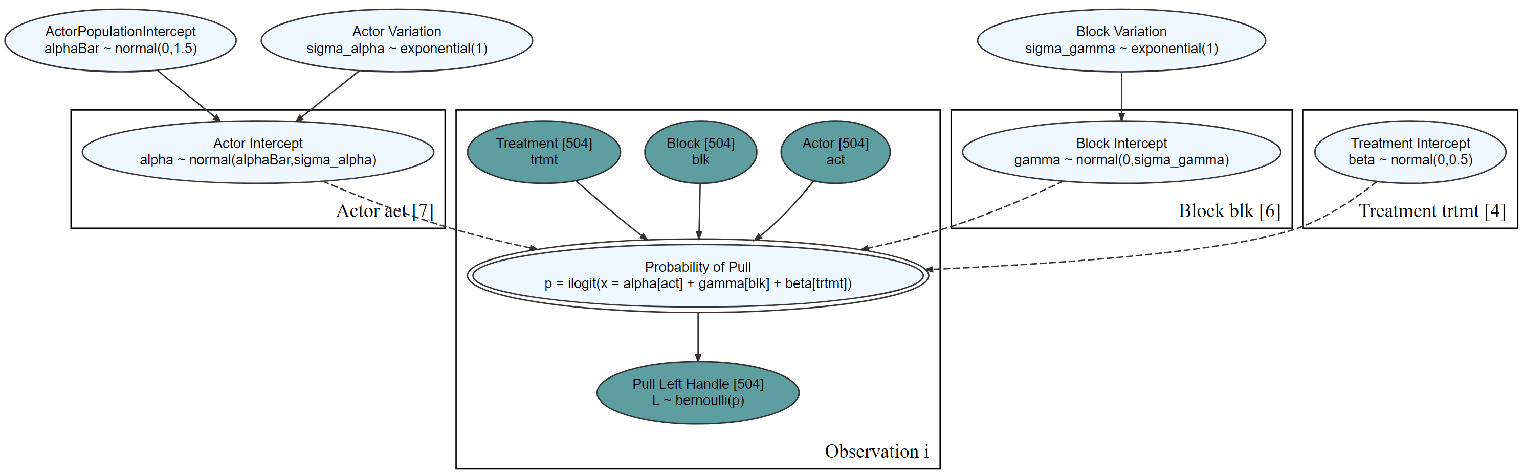
graph %>% dag_render(shortLabel = TRUE)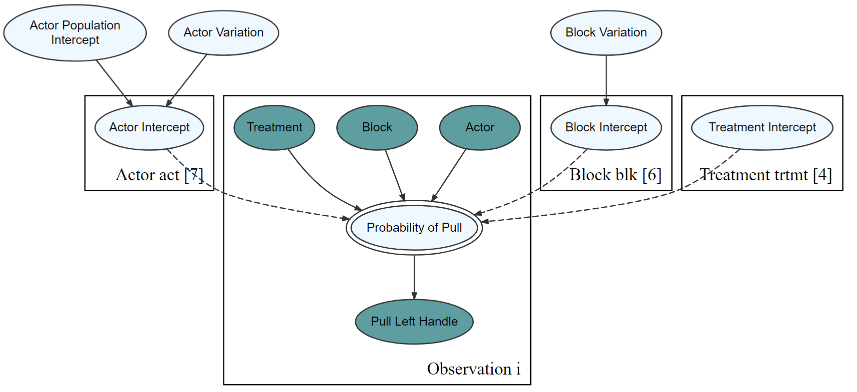
drawsDF = graph %>% dag_numpyro()drawsDF %>% dagp_plot()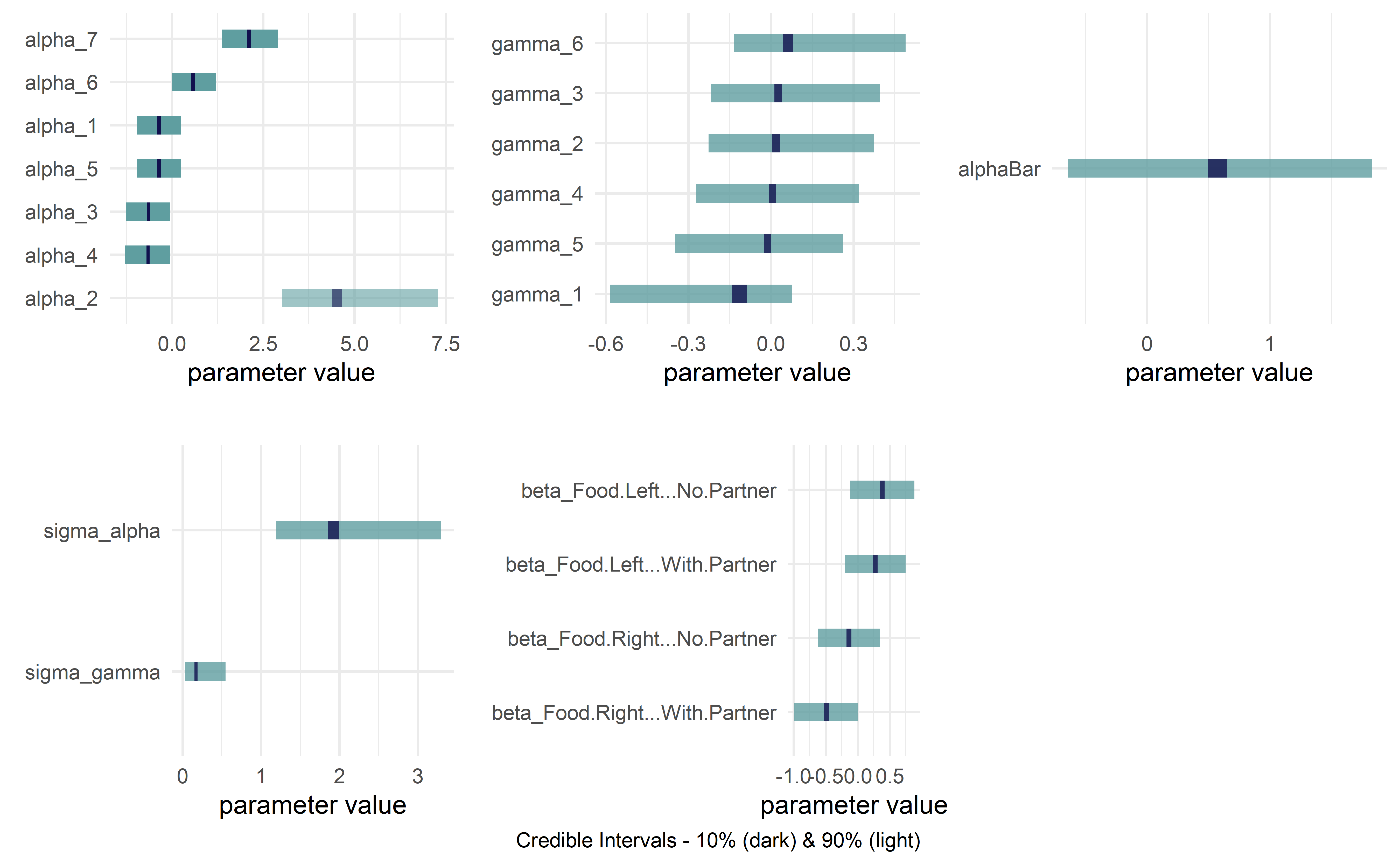
Gelman, Andrew, Hal S. Stern, John B. Carlin, David B. Dunson, Aki Vehtari, and Donald B. Rubin. Bayesian data analysis. Chapman and Hall/CRC, 2013.
library(tidyverse)
library(causact)

# data object used below, schoolDF, is built-in to causact package

graph = dag_create() %>%
  dag_node("Treatment Effect","y",
           rhs = normal(theta, sigma),
           data = causact::schoolsDF$y) %>%
  dag_node("Std Error of Effect Estimates","sigma",
           data = causact::schoolsDF$sigma,
           child = "y") %>%
  dag_node("Exp. Treatment Effect","theta",
           child = "y",
           rhs = avgEffect + schoolEffect) %>%
  dag_node("Pop Treatment Effect","avgEffect",
           child = "theta",
           rhs = normal(0,30)) %>%
  dag_node("School Level Effects","schoolEffect",
           rhs = normal(0,30),
           child = "theta") %>%
  dag_plate("Observation","i",nodeLabels = c("sigma","y","theta")) %>%
  dag_plate("School Name","school",
            nodeLabels = "schoolEffect",
            data = causact::schoolsDF$schoolName,
addDataNode = TRUE)graph %>% dag_render()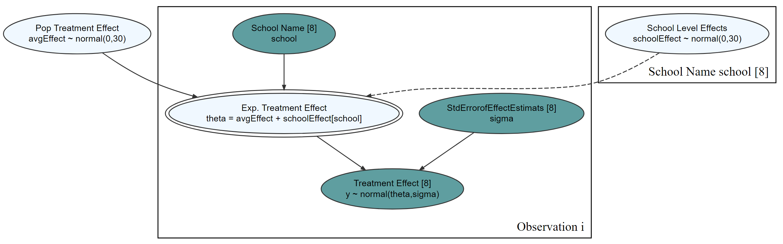
drawsDF = graph %>% dag_numpyro()drawsDF %>% dagp_plot()