![]()
![]()
A set of tools for Bayesian nonparametric density estimation using Martingale posterior distributions including the Copula Resampling (CopRe) algorithm. Also included are a Gibbs sampler for the marginal Gibbs-type mixture model and an extension to include full uncertainty quantification via a predictive Sequence Resampling (SeqRe) algorithm. The CopRe and SeqRe samplers generate random nonparametric distributions as output, leading to complete nonparametric inference on posterior summaries. Routines for calculating arbitrary functionals from the sampled distributions are included as well as an important algorithm for finding the number and location of modes, which can then be used to estimate the clusters in the data.
You can install the latest stable development version of CopRe from GitHub with:
# install.packages("devtools")
devtools::install_github("blakemoya/copre")The basic usage of CopRe for density estimation is to supply a data vector, a number of forward simulations per sample, and a number of samples to draw:
library(copre)
data <- sample(c(rnorm(100, mean = -2), rnorm(100, mean = 2)))
res_cop <- copre(data, 250, 100)
plot(res_cop) +
  geom_function(
    fun = function(x) (dnorm(x, mean = -2) + dnorm(x, mean = 2)) / 2
    )
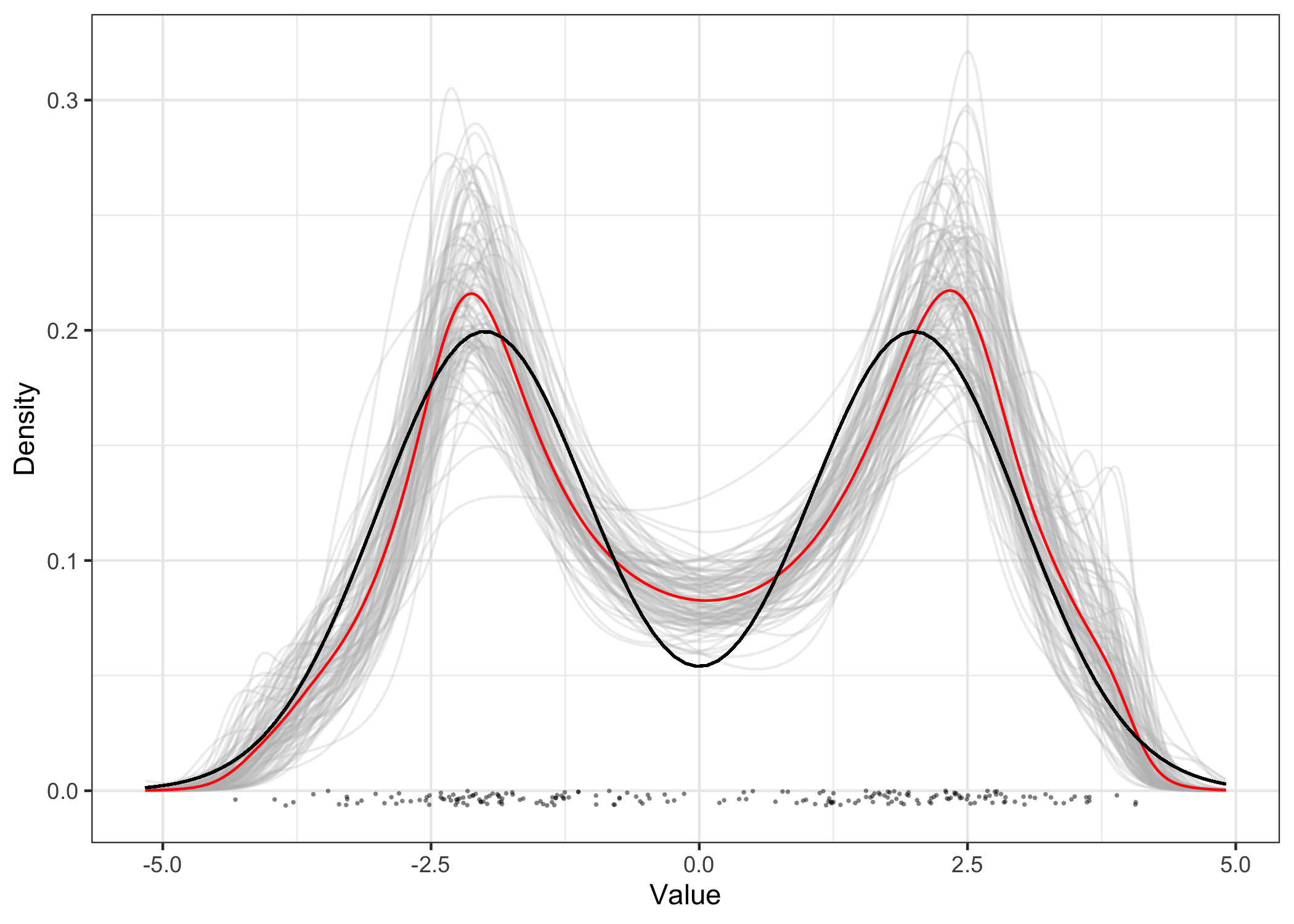
Currently only a Gaussian kernel copula is supported but more options are to be added in future versions.
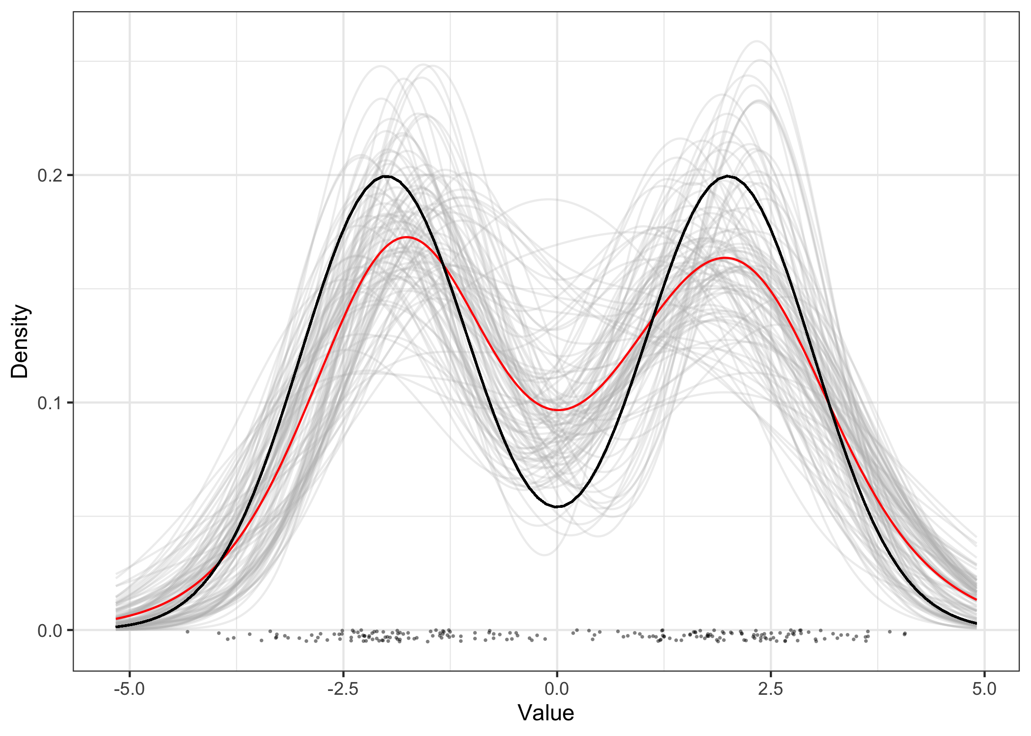
Using SeqRe first involves specifying a model via a base measure
G and an exchangeable sequence measure Sq.
Here we can set up a normal location scale mixture with components
assigned according to a Dirichlet process.
We can then fit the marginal mixture model with the
gibbsmix MCMC routine and then extend the results to their
full nonparametric potential via seqre.
b_norm <- G_normls()
s_dp <- Sq_dirichlet()

res_seq <- gibbsmix(data, 100, b_norm, s_dp) |> seqre()
plot(res_seq) +
  geom_function(
    fun = function(x) (dnorm(x, mean = -2) + dnorm(x, mean = 2)) / 2
    )
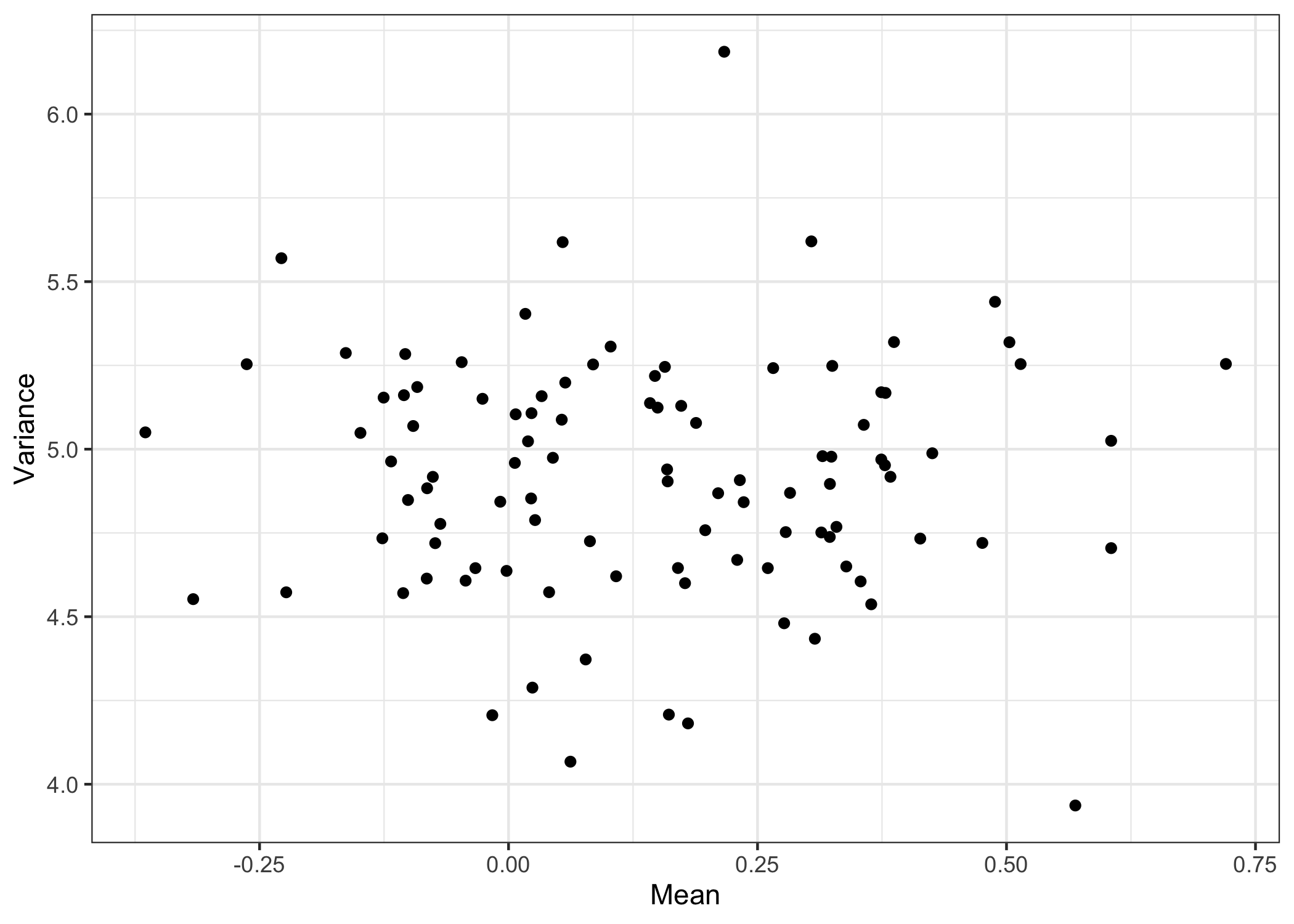
The moments of the estimated distributions can be obtained by calling
moment, and arbitrary functionals of interest can be
obtained similarly with functionals.
moms <- data.frame(Mean = moment(res_cop, 1),
                   Variance = moment(res_cop, 2))
with(moms,
     qplot(Mean, Variance) +
       theme_bw()
     )
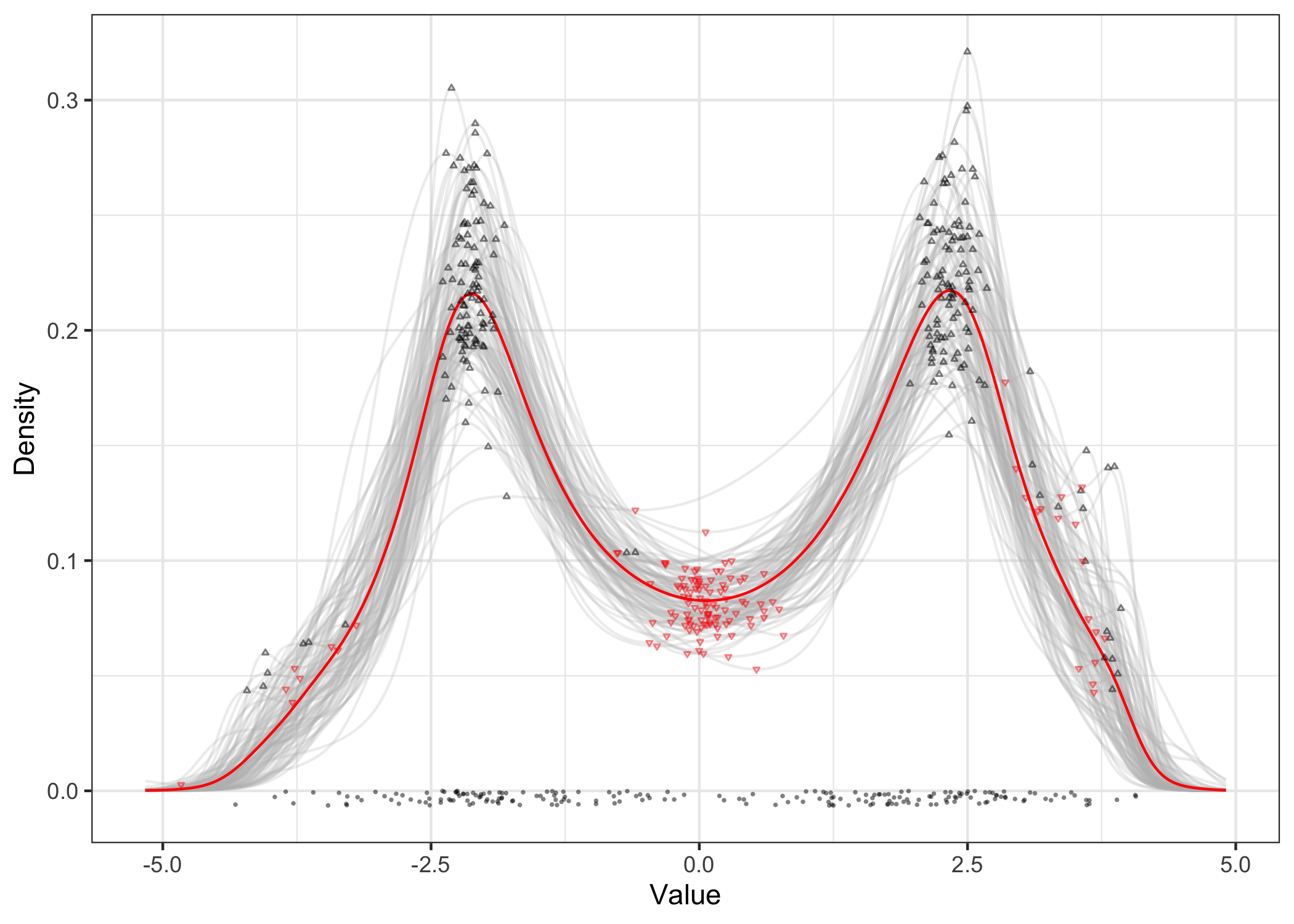
The function modes can be used to isolate local maxima
and minima in the density estimates. Here we can see the detected modes
in black and the antimodes in red. Experiment with using sample
antimodes as a distribution over cluster boundaries!
res_cop.dens <- grideval(res_cop)
ns <- modes(res_cop.dens, idx = TRUE)
us <- antimodes(res_cop.dens, idx = TRUE)
p <- plot(res_cop.dens)
for (i in 1:length(res_cop)) {
  p <- p +
    geom_point(data = data.frame(x = ns[[i]]$value,
                                 y = res_cop.dens[i, ns[[i]]$idx]),
               aes(x = x, y = y), shape = 24, size = 0.5, alpha = 0.5) +
    geom_point(data = data.frame(x = us[[i]]$value,
                                 y = res_cop.dens[i, us[[i]]$idx]),
               aes(x = x, y = y), shape = 25, size = 0.5, alpha = 0.5,
               color = 'red')
}
print(p)
If you have encounter any bugs or other problems while using CopRe, let me know using the Issues tab. For new feature requests, contact me via email at blakemoya@utexas.edu.