
cspp is a package designed to allow a user with only
basic knowledge of R to find variables on state politics and policy,
create and export datasets from these variables, subset the datasets by
states and years, create map visualizations, and export citations to
common file formats (e.g., .bib). An associated web
application is available here.
– Added integration with csppData to allow use of the
most recent CSPP data (version 2.4)
– Added the corr_plot function which allows the creation
of correlation plots and correlation matrices.
– Added the plot_panel function which facilitates the
creation of timeseries plots.
– Added the core argument to the
get_cspp_data function. Set it to TRUE to
merge in common and important variables from the CSPP data. Useful for
teaching purposes.
– Added integration with csppData, a package we created to hold the Correlates of State Policy Project data and codebook. The CSPP data is not provided with this package now. It instead automatically loads the csppData package and its data.
The Correlates of State Policy Project compiles more than 2,000 variables across 50 states (+ DC) from 1900-2020. The variables cover 16 broad categories:
# For latest developmental verison:
library(devtools)
devtools::install_github("correlatesstatepolicy/cspp")

# For CRAN version:
install.packages("cspp")
The primary functions in this package are get_var_info
and get_cspp_data. The basic workflow for using this
package is to 1) find variables of interest and 2) pull them from the
full data into a dataframe within the R environment. Below is a basic
working example.
# Load the package
library(cspp)

# Find variables based on a category
demo_variables <- get_var_info(categories = "demographics")

# Use these variables to get a full or subsetted version of the data
cspp_data <- get_cspp_data(vars = demo_variables$variable,
                           years = seq(2000, 2010))
The get_cspp_data function returns a properly formatted
state-year panel, facilitating regressions and merging based on common
state identifiers.
library(dplyr)
glimpse(cspp_data[1:15],)
#> Rows: 561
#> Columns: 15
#> $ st            <chr> "AK", "AK", "AK", "AK", "AK", "AK", "AK", "AK", "AK", "A…
#> $ stateno       <dbl> 2, 2, 2, 2, 2, 2, 2, 2, 2, 2, 2, 1, 1, 1, 1, 1, 1, 1, 1,…
#> $ state         <chr> "Alaska", "Alaska", "Alaska", "Alaska", "Alaska", "Alask…
#> $ state_fips    <dbl> 2, 2, 2, 2, 2, 2, 2, 2, 2, 2, 2, 1, 1, 1, 1, 1, 1, 1, 1,…
#> $ state_icpsr   <dbl> 81, 81, 81, 81, 81, 81, 81, 81, 81, 81, 81, 41, 41, 41, …
#> $ year          <dbl> 2000, 2001, 2002, 2003, 2004, 2005, 2006, 2007, 2008, 20…
#> $ poptotal      <dbl> 627428, 633160, 642391, 650426, 660975, 668625, 676301, …
#> $ popdensity    <dbl> NA, NA, NA, NA, NA, NA, NA, NA, NA, NA, NA, NA, NA, NA, …
#> $ popfemale     <dbl> 302820, NA, 310665, 313539, 316525, 320479, 323642, 3286…
#> $ pctpopfemale  <dbl> NA, NA, NA, NA, NA, NA, NA, NA, NA, NA, NA, NA, NA, NA, …
#> $ popmale       <dbl> 324112, NA, 333121, 335279, 338910, 343182, 346411, 3548…
#> $ pctpopmale    <dbl> NA, NA, NA, NA, NA, NA, NA, NA, NA, NA, NA, NA, NA, NA, …
#> $ popunder5     <dbl> 47591, NA, 49477, 48680, 49758, 50741, 49771, 51311, 520…
#> $ pctpopunder14 <dbl> NA, NA, NA, NA, NA, NA, NA, NA, NA, NA, NA, NA, NA, NA, …
#> $ pop5to17      <dbl> 143126, NA, 142951, 140609, 138471, 137583, 131663, 1309…
Even more generally, you can load the entire set of variables and/or the entire set of data (all 900+ variables) into R through passing these functions without any parameters:
# All variables
all_variables <- get_var_info()

# Full dataset
all_data <- get_cspp_data()
#> Note: the following variables have additional footnotes in the codebook (https://ippsr.msu.edu/sites/default/files/CorrelatesCodebook.pdf):
#> bfh_cpi_multiplier, gov_fin_fy, housing_prices_quar, noofvotes, cartheftrate, carthefttotal, murderrate, murdertotal, propcrimerate, propcrimetotal, raperate, rapetotal, bus_energy_consum, bus_energy_consum_pcGiven the large number of variables in the data, we provide
additional functionality within get_var_info to search for
variables based on strings or categories. For instance, the following
searches for pop and femal within the variable
name, returning 31 variables:
# Search for variables by name
get_var_info(var_names = c("pop","femal")) %>% dplyr::glimpse()
#> Rows: 43
#> Columns: 14
#> $ variable        <chr> "poptotal", "popdensity", "popfemale", "pctpopfemale",…
#> $ years           <chr> "1900-2019", "1975-1999", "1994-2000, 2002-2010", "201…
#> $ short_desc      <chr> "Population total", "Population density", "Female popu…
#> $ long_desc       <chr> "Total population per state", "Number of people per sq…
#> $ sources         <chr> "U.S. Census Bureau (http://www.census.gov/)\r\nOrigin…
#> $ category        <chr> "demographics", "demographics", "demographics", "demog…
#> $ plaintext_cite  <chr> "Stateminder: A data visualization project from George…
#> $ bibtex_cite     <chr> "@misc{stateminderNA,\n  title={Stateminder.org},\n  a…
#> $ plaintext_cite2 <chr> NA, NA, NA, NA, NA, NA, NA, NA, NA, NA, NA, NA, NA, NA…
#> $ bibtex_cite2    <chr> NA, NA, NA, NA, NA, NA, NA, NA, NA, NA, NA, NA, NA, NA…
#> $ plaintext_cite3 <chr> NA, NA, NA, NA, NA, NA, NA, NA, NA, NA, NA, NA, NA, NA…
#> $ bibtex_cite3    <chr> NA, NA, NA, NA, NA, NA, NA, NA, NA, NA, NA, NA, NA, NA…
#> $ plaintext_cite4 <chr> NA, NA, NA, NA, NA, NA, NA, NA, NA, NA, NA, NA, NA, NA…
#> $ bibtex_cite4    <chr> NA, NA, NA, NA, NA, NA, NA, NA, NA, NA, NA, NA, NA, NA…
A similar line of code using the related_to parameter,
instead of var_name, searches within the name
and the description fields, returning 96 results:
# Search by name and description:
get_var_info(related_to = c("pop", "femal")) %>% dplyr::glimpse()
#> Rows: 139
#> Columns: 14
#> $ variable        <chr> "poptotal", "popdensity", "popfemale", "pctpopfemale",…
#> $ years           <chr> "1900-2019", "1975-1999", "1994-2000, 2002-2010", "201…
#> $ short_desc      <chr> "Population total", "Population density", "Female popu…
#> $ long_desc       <chr> "Total population per state", "Number of people per sq…
#> $ sources         <chr> "U.S. Census Bureau (http://www.census.gov/)\r\nOrigin…
#> $ category        <chr> "demographics", "demographics", "demographics", "demog…
#> $ plaintext_cite  <chr> "Stateminder: A data visualization project from George…
#> $ bibtex_cite     <chr> "@misc{stateminderNA,\n  title={Stateminder.org},\n  a…
#> $ plaintext_cite2 <chr> NA, NA, NA, NA, NA, NA, NA, NA, NA, NA, NA, NA, NA, NA…
#> $ bibtex_cite2    <chr> NA, NA, NA, NA, NA, NA, NA, NA, NA, NA, NA, NA, NA, NA…
#> $ plaintext_cite3 <chr> NA, NA, NA, NA, NA, NA, NA, NA, NA, NA, NA, NA, NA, NA…
#> $ bibtex_cite3    <chr> NA, NA, NA, NA, NA, NA, NA, NA, NA, NA, NA, NA, NA, NA…
#> $ plaintext_cite4 <chr> NA, NA, NA, NA, NA, NA, NA, NA, NA, NA, NA, NA, NA, NA…
#> $ bibtex_cite4    <chr> NA, NA, NA, NA, NA, NA, NA, NA, NA, NA, NA, NA, NA, NA…
You can also return whole categories of variables. The full list of
variable categories is available within the help file for
?get_cspp_data. You can alternatively see the list of
categories through the below snippet of code.
# See variable categories:
unique(get_var_info()$category)
#>  [1] "demographics"     "economic-fiscal"  "government"       "elections"
#>  [5] "policy-ideology"  "criminal justice" "education"        "healthcare"
#>  [9] "welfare"          "rights"           "environment"      "drug-alcohol"
#> [13] "gun control"      "labor"            "transportation"   "misc. regulation"
# Find variables by category:
var_cats <- get_var_info(categories = c("gun control", "labor"))You can then use the variable column in this dataframe to pull data
from get_cspp_data through var_cats$variable,
an example of which is below.
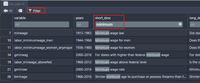
Another option in finding a variable is to load the variables into a dataframe and use RStudio’s filter feature to search:
The function get_cspp_data takes the following
parameters, all of which are optional:
vars - The specific (exact match) variable(s) to pull.
Takes a single variable or a vector of variable names.var_category - The category or categories from which to
pull. Takes a single category or vector of categories from the 16 listed
above.states - Select which states to grab data from. States
must be abbreviated and can take a vector or individual state. See
?state.abb for an easy way to load state
abbreviations.years - Takes a single year or a vector or sequence of
years, such as seq(2001, 2005).output - Choose to write the resulting dataframe
straight to a file. Optional outputs include csv,
dta, or rdata.path - If outputting the file, choose where to write it
to. If left blank, the file will save to your working directory.In this example, the resulting dataframe includes the variables
c("sess_length", "hou_majority", "term_length") as well as
all variables in the category demographics for North
Carolina, Virgina, and Georgia from 1994 to 2004.
# Get subsetted data and save to dataframe
data <- get_cspp_data(vars = c("sess_length", "hou_majority", "term_length"),
                      var_category = "demographics",
                      states = c("NC", "VA", "GA"),
                      years = seq(1995, 2004))
You can also pass the get_var_info function into the
vars parameter of get_cspp_data, skipping a
step:
# Use get_var_info to generate variable vector inline
get_cspp_data(vars = get_var_info(related_to = "concealed carry")$variable,
              states = "NC",
              years = 1999)
#> # A tibble: 1 × 8
#>   st    stateno state          state_fips state_icpsr  year bjourn bprecc
#>   <chr>   <dbl> <chr>               <dbl>       <dbl> <dbl>  <dbl>  <dbl>
#> 1 NC         33 North Carolina         37          47  1999      2      1
Where the two returned variables, bjourn and
bprecc, deal with concealed carry of guns in motor vehicles
and whether state laws pre-empt local laws, respectively.
Each variable in the CSPP data was collected from external sources.
We’ve made it easy to cite the source of each variable you use with the
get_cites function.
This function takes a variable name or vector of variable names (such
as that generated by the get_var_info function) and returns
a dataframe of citations.
# Simple dataframe for one variable
get_cites(var_names = "poptotal") %>% dplyr::glimpse()
#> Rows: 3
#> Columns: 12
#> $ variable        <chr> "poptotal", "cspp_dataset", "cspp_package"
#> $ plaintext_cite  <chr> "Stateminder: A data visualization project from George…
#> $ bibtex_cite     <chr> "@misc{stateminderNA,\n  title={Stateminder.org},\n  a…
#> $ plaintext_cite2 <chr> NA, NA, NA
#> $ bibtex_cite2    <chr> NA, NA, NA
#> $ plaintext_cite3 <chr> NA, NA, NA
#> $ bibtex_cite3    <chr> NA, NA, NA
#> $ years           <chr> "1900-2019", NA, NA
#> $ short_desc      <chr> "Population total", NA, NA
#> $ long_desc       <chr> "Total population per state", NA, NA
#> $ sources         <chr> "U.S. Census Bureau (http://www.census.gov/)\r\nOrigin…
#> $ category        <chr> "demographics", NA, NA

# Using get_var_info to return variable citations
cite_ex <- get_cites(var_names = get_var_info(related_to = "concealed carry")$variable)
cite_ex$plaintext_cite[3:4]
#> [1] "Jordan, Marty P. and Matt Grossmann. 2020. The Correlates of State Policy Project v.2.2. East Lansing, MI: Institute for Public Policy and Social Research (IPPSR)."
#> [2] "Caleb Lucas and Joshua McCrain (2020). cspp: A Package for The Correlates of State Policy Project Data. R package version 0.1.0."
There is also an option to output the citations to a .bib, .csv or .txt file:
get_cites(var_names = "poptotal",
         write_out = TRUE,
         file_path = "~/path/to/file.csv",
format = "csv")The generate_map function uses the CSPP data to generate
US maps with states filled in based on the value of a given variable
(also called choropleths). This function returns a ggplot
object so it is highly customizable. The optional parameters are:
cspp_data - A dataframe ideally generated by the
get_cspp_data function. Any dataframe will work as long as
it has the columns st.abb, year, and any
additional column from which to fill in the map.var_name - The specific variable to use to fill in the
map. If left blank, it will take the first column after
year and st.abb.average_years - Default is FALSE. If set to TRUE, this
returns a map that averages over all of the years per state in the
dataframe. So if there are multiple years of population per state, it
plots the average population per state in the panel.drop_NA_states - By default, the function keeps states
that are missing data, resulting in them being filled in as gray. If
this is set to TRUE, the states are dropped. See the example below.poly_args - A list of arguments that determine the
aesthetics of state shapes. See ggplot2::geom_polygon for
options.Note: This function will attempt to plot any variable type; however, plotting character or factor values on a map will likely result in a hard to interpret graph.
library(ggplot2) # optional, but needed to remove legend

# Generates a map of the percentage of the population over 65
generate_map(get_cspp_data(var_category = "demographics"),
             var_name = "pctpopover65") +
  ggplot2::theme(legend.position = "none")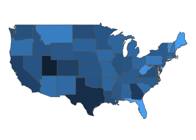
In this example, since the dataframe passed is generated by
get_cspp_data(var_category = "demographics") and contains
all years for all states in the data, the function by default returns
the value of the most recent year without missing data.
If you set drop_NA_states to TRUE, and pass the function
a dataframe containing only certain states, it only plots those
states:
library(dplyr)

generate_map(get_cspp_data(var_category = "demographics") %>%
                dplyr::filter(st %in% c("NC", "VA", "SC")),
              var_name = "pctpopover65",
              poly_args = list(color = "black"),
              drop_NA_states = TRUE) +
  ggplot2::theme(legend.position = "none")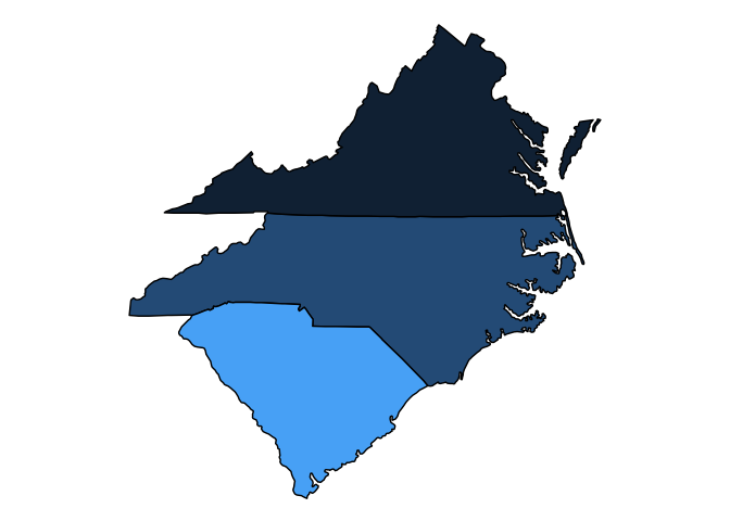
Since this function returns a ggplot object, you can
customize it endlessly:
generate_map(get_cspp_data(var_category = "demographics") %>%
                dplyr::filter(st %in% c("NC", "VA", "SC", "TN", "GA", "WV", "MS", "AL", "KY")),
              var_name = "pctpopover65",
              poly_args = list(color = "black"),
              drop_NA_states = TRUE) +
  ggplot2::scale_fill_gradient(low = "white", high = "red") +
  ggplot2::theme(legend.position = "none") +
  ggplot2::ggtitle("% Population Over 65")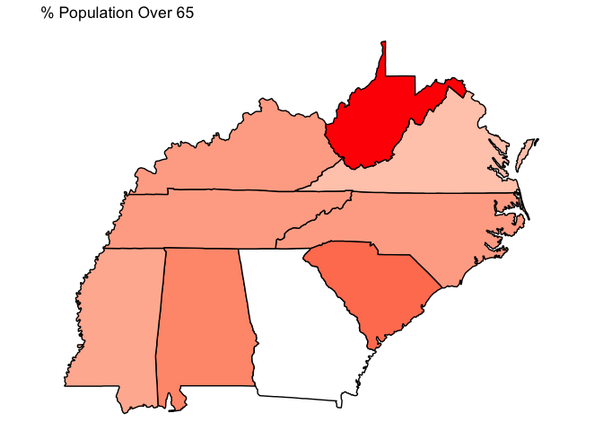
To facilitate the visualization of the timeseries and panel nature of
the CSPP data, the plot_panel function takes a dataframe
from get_cspp_data and plots a state-year panel in one of
two formats. The parameters of this function are as follows:
cspp_data - a dataframe generated by
get_cspp_data or, alternatively, a dataframe with the
columns st.abb, year, plus one other
variable.var_name - the name of the variable to be plotted.years - the years to include in the panel.colors - three color values that are used in the plot.
The first color takes the lowest values of the variable, the second the
highest, and the third is the color used for NA values.plot_type - one of “grid” or “line”. Defaults to
“grid”. Both are displayed next.The function returns a ggplot2 object, making it easier
to change and add layers onto the generated plot.
A common research design is to use variation in policy adoption as a ‘treatment’ in a pseudo-experimental setting. This function makes it easy to visualize when states are subject to this treatment.
# panel of all states' adoption of medical marijuana laws
cspp <- get_cspp_data(vars = "drugs_medical_marijuana")

# visualize panel:
plot_panel(cspp)
#> Values from drugs_medical_marijuana used to fill cells.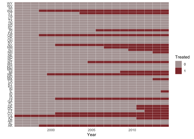
The function also works with continuous variables, such as the state policy liberalism score:
plot_panel(cspp_data = get_cspp_data(vars = "pollib_median"),
           colors = c("firebrick4", "steelblue2", "gray"),
           years = seq(1960, 2010)) +
  ggplot2::ggtitle("Policy liberalism")
#> Values from pollib_median used to fill cells.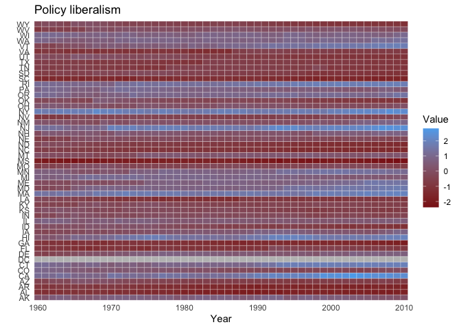
The corr_plot function geneates a correlation plot (in
the style of a heat map) using ggcorrplot. Alternately, it
outputs a correlation matrix for users to pass onto their own
ggcorrplot call for further customization.
This function takes the following parameters: * data - a
dataframe. If generated by get_cspp_data, the function will
work automatically. Otherwise, this function parses all numeric columns
in the passed dataframe. * vars- a vector of variable names
to generate correlations between. * summarize - whether to
create state specific means for each variable. If set to TRUE, passed
dataframe must contain the column st.abb. If FALSE, it will
treat each observation independently in generating correlations. *
labels - whether to include labels on the correlation plot
of the specific correlation value. * label_size - the font
size of the labels. * colors - a vector of three colors
that form the gradient in the plot. * cor_matrix - if set
to TRUE, instead of returning a ggplot object this function returns a
correlation matrix.
corr_plot(data = get_cspp_data(years = seq(1990, 2010)),
vars = c("pollib_median", "innovatescore_boehmkeskinner", "citi6013", "ranney4_control", "h_diffs"),
colors = c("dodgerblue", "white", "firebrick"))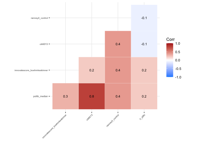 Alternatively, you can use similar code to generate a correlation
matrix:
Alternatively, you can use similar code to generate a correlation
matrix:
corr_plot(data = get_cspp_data(years = seq(1990, 2010)),
          vars = c("pollib_median", "innovatescore_boehmkeskinner", "citi6013", "ranney4_control", "h_diffs"),
          cor_matrix = TRUE)
#>                              pollib_median innovatescore_boehmkeskinner
#> pollib_median                          1.0                          0.3
#> innovatescore_boehmkeskinner           0.3                          1.0
#> citi6013                               0.8                          0.2
#> ranney4_control                        0.4                          0.4
#> h_diffs                                0.2                          0.2
#>                              citi6013 ranney4_control h_diffs
#> pollib_median                     0.8             0.4     0.2
#> innovatescore_boehmkeskinner      0.2             0.4     0.2
#> citi6013                          1.0             0.4    -0.1
#> ranney4_control                   0.4             1.0    -0.1
#> h_diffs -0.1 -0.1 1.0The function get_network_data returns a dataset from the
CSPP state
networks data consisting of 120 variables. The data is structured as
state dyads (an edge list).
# Returns dataframe of state dyads
get_network_data() %>% dplyr::glimpse()
#> Rows: 2,550
#> Columns: 120
#> $ State1                     <chr> "Alabama", "Alabama", "Alabama", "Alabama",…
#> $ State2                     <chr> "Alaska", "Arizona", "Arkansas", "Californi…
#> $ st.abb2                    <chr> "AK", "AZ", "AR", "CA", "CO", "CT", "DE", "…
#> $ st.abb1                    <chr> "AL", "AL", "AL", "AL", "AL", "AL", "AL", "…
#> $ dyadid                     <chr> "AL-AK", "AL-AZ", "AL-AR", "AL-CA", "AL-CO"…
#> $ S1region                   <chr> "South", "South", "South", "South", "South"…
#> $ S2region                   <chr> "West", "West", "South", "West", "West", "N…
#> $ S1division                 <chr> "East South Central", "East South Central",…
#> $ S2division                 <chr> "Pacific", "Mountain", "West South Central"…
#> $ Border                     <dbl> 0, 0, 0, 0, 0, 0, 0, 0, 1, 1, 0, 0, 0, 0, 0…
#> $ Distance                   <dbl> 4594.3668, 2407.6648, 620.4273, 3243.6837, …
#> $ State1_Lat                 <dbl> 32.36154, 32.36154, 32.36154, 32.36154, 32.…
#> $ State1_Long                <dbl> -86.27912, -86.27912, -86.27912, -86.27912,…
#> $ State2_Lat                 <dbl> 58.30194, 33.44846, 34.73601, 38.55560, 39.…
#> $ State2_Long                <dbl> -134.41974, -112.07384, -92.33112, -121.468…
#> $ ACS_Migration              <dbl> 528, 1005, 926, 3107, 1251, 327, 113, 99, 1…
#> $ PopDif                     <dbl> 4088469, -2116015, 1850948, -34266641, -722…
#> $ State1_Pop                 <dbl> 4819343, 4819343, 4819343, 4819343, 4819343…
#> $ State2_Pop                 <dbl> 730874, 6935358, 2968395, 39085984, 5542282…
#> $ IncomingFlights            <dbl> 75, 0, 0, 72, 51, 328, 0, 0, 0, 606, 0, 77,…
#> $ IRS_migration              <dbl> 7698, 15051, 17858, 61401, 19956, 6408, 252…
#> $ Income                     <dbl> 147372, 339243, 371553, 1364538, 445755, 18…
#> $ IRS_migration_2010         <dbl> 528, 1005, 926, 3107, 1251, 327, 113, 99, 1…
#> $ Income_2010                <dbl> 9214, 23289, 18692, 66991, 25235, 9019, 236…
#> $ Imports                    <dbl> 2.997198e+05, 2.065025e+09, 2.033900e+09, 4…
#> $ GSPDif                     <dbl> 155221, -100224, 84242, -2417106, -117019, …
#> $ S1GSP                      <dbl> 205625, 205625, 205625, 205625, 205625, 205…
#> $ S2GSP                      <dbl> 50404, 305849, 121383, 2622731, 322644, 259…
#> $ DemDif                     <dbl> -0.07857143, -0.14523810, -0.06571428, -0.3…
#> $ S1AvgDem                   <dbl> 0.2714286, 0.2714286, 0.2714286, 0.2714286,…
#> $ S2AvgDem                   <dbl> 0.3500000, 0.4166667, 0.3371429, 0.6375000,…
#> $ S1SenDemProp               <dbl> 0.2285714, 0.2285714, 0.2285714, 0.2285714,…
#> $ S1HSDemProp                <dbl> 0.3142857, 0.3142857, 0.3142857, 0.3142857,…
#> $ S2SenDemProp               <dbl> 0.3000000, 0.4333333, 0.3142857, 0.6250000,…
#> $ S2HSDemProp                <dbl> 0.4000000, 0.4000000, 0.3600000, 0.6500000,…
#> $ IdeologyDif                <dbl> 0.31610168, 0.06866579, -0.11840535, -0.213…
#> $ PIDDif                     <dbl> 0.14324945, -0.10957587, -0.15900619, -0.27…
#> $ S1Ideology                 <dbl> -0.03389831, -0.03389831, -0.03389831, -0.0…
#> $ S1PID                      <dbl> -0.3304348, -0.3304348, -0.3304348, -0.3304…
#> $ S2Ideology                 <dbl> -0.34999999, -0.10256410, 0.08450704, 0.179…
#> $ S2PID                      <dbl> -0.47368422, -0.22085890, -0.17142858, -0.0…
#> $ policy_diffusion_tie       <dbl> 0, 20, 7, 5, 1, 5, 56, NA, 15, 40, 0, 19, 5…
#> $ policy_diffusion_2015      <dbl> 0, 1, 0, 1, 0, 0, 1, NA, 1, 1, 0, 1, 1, 0, …
#> $ policy_diffusion_2000.2015 <dbl> 0, 7, 0, 5, 0, 3, 16, NA, 13, 16, 0, 16, 15…
#> $ LibDif                     <dbl> NA, 34.186113, 2.949804, 46.088120, 44.4234…
#> $ ELibDif                    <dbl> NA, 1.230781, -2.156186, -3.115099, 8.00975…
#> $ SLibDif                    <dbl> NA, -32.955332, -0.793618, -42.973021, -36.…
#> $ S1EconomicLiberalism       <dbl> -0.0384034, -0.0384034, -0.0384034, -0.0384…
#> $ S1SocialLiberalism         <dbl> -0.2714913, -0.2714913, -0.2714913, -0.2714…
#> $ S2EconomicLiberalism       <dbl> NA, -0.05071121, -0.01684154, -0.00725241, …
#> $ S2SocialLiberalism         <dbl> NA, 0.05806200, -0.26355514, 0.15823889, 0.…
#> $ MassSocLibDif              <dbl> -0.38336566, 0.08869284, -1.38085590, -2.22…
#> $ MassEconLibDif             <dbl> -0.06364249, -0.14963306, -0.07359393, -0.5…
#> $ PolSocLibDif               <dbl> -1.4865111, 0.2728079, -0.9492451, -4.20959…
#> $ PolEconLibDif              <dbl> -1.1890527, -0.2309994, -0.1488198, -2.9290…
#> $ State1PolSocLib            <dbl> -1.577025, -1.577025, -1.577025, -1.577025,…
#> $ State1PolEconLib           <dbl> -1.370212, -1.370212, -1.370212, -1.370212,…
#> $ State1MassSocLib           <dbl> 0.07021931, 0.07021931, 0.07021931, 0.07021…
#> $ State1MassEconLib          <dbl> -0.5247536, -0.5247536, -0.5247536, -0.5247…
#> $ State2PolSocLib            <dbl> -0.090514018, -1.849832972, -0.627779955, 2…
#> $ State2PolEconLib           <dbl> -0.18115938, -1.13921271, -1.22139223, 1.55…
#> $ State2MassSocLib           <dbl> 0.45358497, -0.01847353, 1.45107521, 2.2920…
#> $ State2MassEconLib          <dbl> -0.4611111, -0.3751206, -0.4511597, 0.01890…
#> $ perceived_similarity       <dbl> 0.116279073, 0.067307696, 0.343750000, 0.00…
#> $ RaceDif                    <dbl> 50.6, 66.0, 22.0, 97.9, 44.8, 33.5, 16.7, 5…
#> $ LatinoDif                  <dbl> -2.9, -27.3, -3.3, -35.0, -17.4, -12.0, -5.…
#> $ WhiteDif                   <dbl> 4.9, 10.8, -6.8, 28.5, -2.7, -1.2, 3.3, 29.…
#> $ BlackDif                   <dbl> 23.8, 22.6, 11.5, 21.2, 22.8, 16.8, 5.2, -1…
#> $ AsianDif                   <dbl> -5.3, -1.9, -0.3, -13.1, -1.8, -3.2, -2.7, …
#> $ NativeDif                  <dbl> -13.7, -3.4, -0.1, 0.1, -0.1, 0.3, 0.3, 0.3…
#> $ S1Latino                   <dbl> 0.041, 0.041, 0.041, 0.041, 0.041, 0.041, 0…
#> $ S1White                    <dbl> 0.655, 0.655, 0.655, 0.655, 0.655, 0.655, 0…
#> $ S1Black                    <dbl> 0.267, 0.267, 0.267, 0.267, 0.267, 0.267, 0…
#> $ S1Asian                    <dbl> 0.013, 0.013, 0.013, 0.013, 0.013, 0.013, 0…
#> $ S1Native                   <dbl> 0.005, 0.005, 0.005, 0.005, 0.005, 0.005, 0…
#> $ S2Latino                   <dbl> 0.070, 0.314, 0.074, 0.391, 0.215, 0.161, 0…
#> $ S2White                    <dbl> 0.606, 0.547, 0.723, 0.370, 0.682, 0.667, 0…
#> $ S2Black                    <dbl> 0.029, 0.041, 0.152, 0.055, 0.039, 0.099, 0…
#> $ S2Asian                    <dbl> 0.066, 0.032, 0.016, 0.144, 0.031, 0.045, 0…
#> $ S2Native                   <dbl> 0.142, 0.039, 0.006, 0.004, 0.006, 0.002, 0…
#> $ ReligDif                   <dbl> 74, 77, 23, 89, 58, 94, 81, 74, 63, 22, 77,…
#> $ ChristianDif               <dbl> 24, 19, 7, 23, 22, 16, 17, 21, 16, 7, 23, 1…
#> $ EvangelicalDif             <dbl> 27, 23, 3, 29, 23, 36, 34, 35, 25, 11, 24, …
#> $ MainlineDif                <dbl> 1, 1, -3, 3, -2, -4, -8, -2, -1, 1, 2, -3, …
#> $ BPDif                      <dbl> 13, 15, 8, 14, 14, 11, 6, 4, 8, -1, 14, 16,…
#> $ CatholicDif                <dbl> -9, -14, -1, -21, -9, -26, -15, -12, -14, -…
#> $ MormonDif                  <dbl> -4, -4, 0, 0, -1, 0, 1, 0, 0, 0, -2, -18, 1…
#> $ JewishDif                  <dbl> 0, -2, 0, -2, -1, -3, -3, -4, -3, -1, 0, 0,…
#> $ MuslimDif                  <dbl> 0, -1, -2, -1, 0, -1, -1, -2, 0, 0, 0, -1, …
#> $ BuddhistDif                <dbl> -1, -1, 0, -2, -1, -1, 0, -2, 0, 0, -8, 0, …
#> $ HinduDif                   <dbl> 0, -1, 0, -2, 0, -1, -2, -1, 0, 0, 0, 0, -1…
#> $ NonesDif                   <dbl> -19, -15, -6, -15, -7, -11, -11, -12, -12, …
#> $ NPDif                      <dbl> -11, -10, -4, -9, -11, -5, -9, -7, -8, -4, …
#> $ ReligiosityDif             <dbl> 32, 24, 7, 28, 30, 34, 25, 24, 23, 11, 30, …
#> $ S1Christian                <dbl> 0.86, 0.86, 0.86, 0.86, 0.86, 0.86, 0.86, 0…
#> $ S1Evangelical              <dbl> 0.49, 0.49, 0.49, 0.49, 0.49, 0.49, 0.49, 0…
#> $ S1Mainline                 <dbl> 0.13, 0.13, 0.13, 0.13, 0.13, 0.13, 0.13, 0…
#> $ S1BlackProt                <dbl> 0.16, 0.16, 0.16, 0.16, 0.16, 0.16, 0.16, 0…
#> $ S1Catholic                 <dbl> 0.07, 0.07, 0.07, 0.07, 0.07, 0.07, 0.07, 0…
#> $ S1Mormon                   <dbl> 0.01, 0.01, 0.01, 0.01, 0.01, 0.01, 0.01, 0…
#> $ S1Jewish                   <dbl> 0, 0, 0, 0, 0, 0, 0, 0, 0, 0, 0, 0, 0, 0, 0…
#> $ S1Muslim                   <dbl> 0, 0, 0, 0, 0, 0, 0, 0, 0, 0, 0, 0, 0, 0, 0…
#> $ S1Buddhist                 <dbl> 0, 0, 0, 0, 0, 0, 0, 0, 0, 0, 0, 0, 0, 0, 0…
#> $ S1Hindu                    <dbl> 0, 0, 0, 0, 0, 0, 0, 0, 0, 0, 0, 0, 0, 0, 0…
#> $ S1Nones                    <dbl> 0.12, 0.12, 0.12, 0.12, 0.12, 0.12, 0.12, 0…
#> $ S1NothingParticular        <dbl> 0.09, 0.09, 0.09, 0.09, 0.09, 0.09, 0.09, 0…
#> $ S1HighlyReligious          <dbl> 0.77, 0.77, 0.77, 0.77, 0.77, 0.77, 0.77, 0…
#> $ S2Christian                <dbl> 0.62, 0.67, 0.79, 0.63, 0.64, 0.70, 0.69, 0…
#> $ S2Evangelical              <dbl> 0.22, 0.26, 0.46, 0.20, 0.26, 0.13, 0.15, 0…
#> $ S2Mainline                 <dbl> 0.12, 0.12, 0.16, 0.10, 0.15, 0.17, 0.21, 0…
#> $ S2BlackProt                <dbl> 0.03, 0.01, 0.08, 0.02, 0.02, 0.05, 0.10, 0…
#> $ S2Catholic                 <dbl> 0.16, 0.21, 0.08, 0.28, 0.16, 0.33, 0.22, 0…
#> $ S2Mormon                   <dbl> 0.05, 0.05, 0.01, 0.01, 0.02, 0.01, 0.00, 0…
#> $ S2Jewish                   <dbl> 0.00, 0.02, 0.00, 0.02, 0.01, 0.03, 0.03, 0…
#> $ S2Muslim                   <dbl> 0.00, 0.01, 0.02, 0.01, 0.00, 0.01, 0.01, 0…
#> $ S2Buddhist                 <dbl> 0.01, 0.01, 0.00, 0.02, 0.01, 0.01, 0.00, 0…
#> $ S2Hindu                    <dbl> 0.00, 0.01, 0.00, 0.02, 0.00, 0.01, 0.02, 0…
#> $ S2Nones                    <dbl> 0.31, 0.27, 0.18, 0.27, 0.19, 0.23, 0.23, 0…
#> $ S2NothingParticular        <dbl> 0.20, 0.19, 0.13, 0.18, 0.20, 0.14, 0.18, 0…
#> $ S2HighlyReligious          <dbl> 0.45, 0.53, 0.70, 0.49, 0.47, 0.43, 0.52, 0…
The function has two optional parameters category and
merge_data. If a category or string of categories is
specified, it returns variables only in that category (see the data
documentation in the link above). Category options are “Distance Travel
Migration”, “Economic”, “Political”, “Policy”, “Demographic”.
network.df <- get_network_data(category = c("Economic", "Political"))

names(network.df)
#>  [1] "State1"             "State2"             "st.abb2"
#>  [4] "st.abb1"            "dyadid"             "IRS_migration"
#>  [7] "Income"             "IRS_migration_2010" "Income_2010"
#> [10] "Imports"            "GSPDif"             "S1GSP"
#> [13] "S2GSP"              "DemDif"             "S1AvgDem"
#> [16] "S2AvgDem"           "S1SenDemProp"       "S1HSDemProp"
#> [19] "S2SenDemProp"       "S2HSDemProp"        "IdeologyDif"
#> [22] "PIDDif"             "S1Ideology"         "S1PID"
#> [25] "S2Ideology"         "S2PID"
merge_data simplifies merging in data from the
get_cspp_data function. The object passed to
merge_data must be a dataframe with a variable named
st.abb, or a dataframe generated by
get_cspp_data. If the dataframe passed to this parameter
has more than one observation per state (a panel) then this function
averages over all values per state prior to merging.
cspp_data <- get_cspp_data(vars = c("sess_length", "hou_majority"), years = seq(1999, 2000))

network.df <- get_network_data(category = "Distance Travel Migration",
                               merge_data  = cspp_data)
#> Warning in get_network_data(category = "Distance Travel Migration", merge_data
#> = cspp_data): There are multiple observations per state in the `data` dataframe.
#> Creating one observation per state (dplyr::summarize()) prior to merging...

names(network.df)
#>  [1] "State1"          "State2"          "st.abb2"         "st.abb1"
#>  [5] "dyadid"          "S1region"        "S2region"        "S1division"
#>  [9] "S2division"      "Border"          "Distance"        "State1_Lat"
#> [13] "State1_Long"     "State2_Lat"      "State2_Long"     "ACS_Migration"
#> [17] "PopDif"          "State1_Pop"      "State2_Pop"      "IncomingFlights"
#> [21] "sess_length"     "hou_majority"

library(dplyr)

cspp_data %>%
  arrange(st) %>%
  head()
#> # A tibble: 6 × 8
#>   st    stateno state    state_fips state_icpsr  year sess_length hou_majority
#>   <chr>   <dbl> <chr>         <dbl>       <dbl> <dbl>       <dbl>        <dbl>
#> 1 AK          2 Alaska            2          81  1999       168.         0.752
#> 2 AK          2 Alaska            2          81  2000        NA          0.752
#> 3 AL          1 Alabama           1          41  1999        60         -0.129
#> 4 AL          1 Alabama           1          41  2000        NA         -0.115
#> 5 AR          4 Arkansas          5          42  1999        63.2        0.118
#> 6 AR          4 Arkansas          5          42  2000        NA          0.118
# the merged value of Alaska's hou_majority value will be mean(c(-0.129, -0.115))Here are two examples of plotting the state network edgelist data
using igraph and ggraph:
library(ggraph)
library(igraph)

network.df <- select(network.df, from = st.abb1, to = st.abb2, ACS_Migration)

network.df %>%
  filter(from %in% c("NC", "VA", "SC", "GA")) %>%
  graph_from_data_frame() %>%
  ggraph(layout="fr") +
  geom_edge_link(aes(edge_alpha = ACS_Migration), edge_color = "royalblue") +
  geom_node_point() +
  geom_node_text(aes(label = name), repel = TRUE, point.padding = unit(0.2, "lines")) +
  theme_void() +
  theme(legend.position = "none")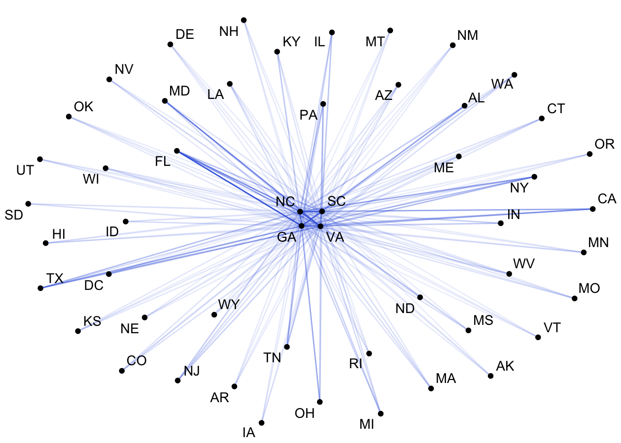
network.df %>%
  filter(from %in% c("NC")) %>%
  graph_from_data_frame() %>%
  ggraph(layout="linear") +
  geom_edge_arc(aes(edge_alpha = ACS_Migration), edge_color = "royalblue") +
  geom_node_text(aes(label = name), size = 2) +
  theme_void() +
  theme(legend.position = "none")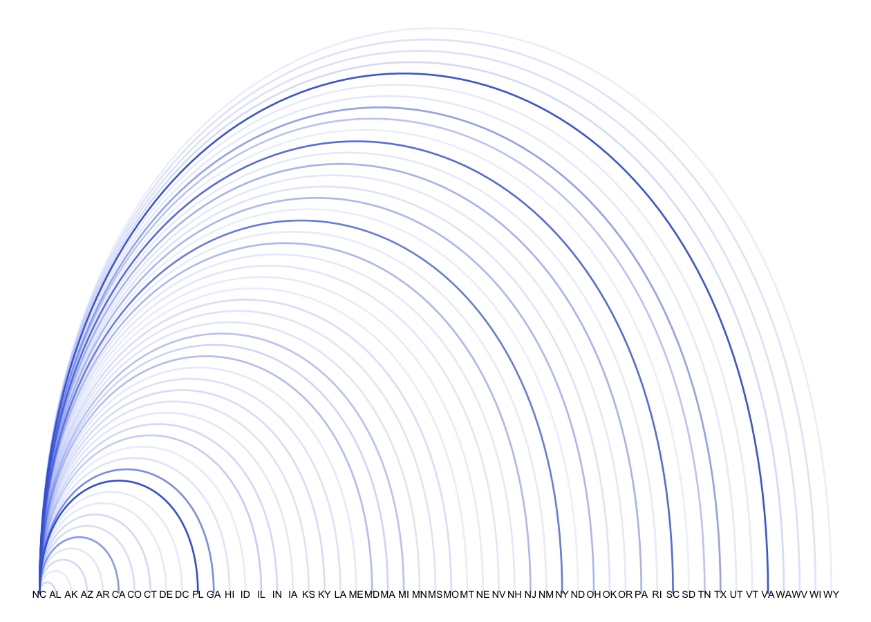
Caleb Lucas and Joshua McCrain (2020). cspp: A Package for The Correlates of State Policy Project Data. R package version 0.3.3.
Caleb Lucas -
Political Scientist, RAND Corporation
Josh McCrain -
Assistant Professor, University of Utah (Twitter)