Luis F. Arias-Giraldo, Marlon E. Cobos, A. Townsend Peterson
![]()
![]()
enmpa is an R package that contains a set of tools to
perform Ecological Niche Modeling using presence-absence data. Some of
the main functions help perform data partitioning, model calibration,
model selection, variable response exploration, and model
projection.
If you use enmpa in your research, please cite the
following paper:
Arias-Giraldo, Luis F., and Marlon E. Cobos. 2024. “enmpa: An R Package for Ecological Niche Modeling Using Presence-Absence Data and Generalized Linear Models”. Biodiversity Informatics 18. https://doi.org/10.17161/bi.v18i.21742.
To install the stable version of enmpa from CRAN
use:
install.packages("enmpa")You can install the development version of enmpa from GitHub with:
# install.packages("remotes")
remotes::install_github("Luisagi/enmpa")The package terra is used to handle spatial data, and
enmpa is used to perform ENM.
library(enmpa)
library(terra)The data used in this example is included in enmpa.
# Species presence absence data associated with environmental variables
data("enm_data", package = "enmpa")

# Data for final model evaluation
data("test", package = "enmpa")

# Environmental data as raster layers for projections
env_vars <- rast(system.file("extdata", "vars.tif", package = "enmpa"))

# Check the example data
head(enm_data)
#>   Sp     bio_1 bio_12
#> 1  0  4.222687    403
#> 2  0  6.006802    738
#> 3  0  4.079385    786
#> 4  1  8.418489    453
#> 5  0  8.573750    553
#> 6  1 16.934618    319
The raster layers for projections were obtained from WorldClim:
plot(env_vars, mar = c(1, 1, 2, 4))
To explore the relevance of the variables to be used in niche models, we implemented in the methods developed by (Cobos and Peterson 2022). These methods help to identify signals of ecological niche considering distinct variables and the presence-absence data. By characterizing the sampling universe, this approach can determine whether presences and absences can be separated better than randomly considering distinct environmental factors.
sn_bio1  <- niche_signal(data = enm_data, variables = "bio_1",
                         condition = "Sp", method = "univariate")

sn_bio12 <- niche_signal(data = enm_data, variables = "bio_12",
condition = "Sp", method = "univariate")plot_niche_signal(sn_bio1, variables = "bio_1")
plot_niche_signal(sn_bio12, variables = "bio_12")

Based on the univariate test results, the variables bio_1 and bio_12 help to detect signals of ecological niche in our data. In our example, the species tends to occur in areas with higher annual mean temperatures (bio_1); whereas, considering annual precipitation (bio_12), the species seems to be present in areas with lower values. See the function’s documentation for more information.
With enmpa you have the possibility to explore multiple
model formulas derived from combinations of variables considering linear
(l), quadratic (q), and product (p) responses. Product refers to pair
interactions of variables.
The function includes the flag mode to determine what
strategy to use to combine predictors based on the responses defined in
. The options of mode are:
An example using linear + quadratic responses:
get_formulas(dependent = "Sp", independent = c("bio_1", "bio_12"),
             type = "lq", mode = "intensive")
#>  [1] "Sp ~ bio_1"
#>  [2] "Sp ~ bio_12"
#>  [3] "Sp ~ I(bio_1^2)"
#>  [4] "Sp ~ I(bio_12^2)"
#>  [5] "Sp ~ bio_1 + bio_12"
#>  [6] "Sp ~ bio_1 + I(bio_1^2)"
#>  [7] "Sp ~ bio_1 + I(bio_12^2)"
#>  [8] "Sp ~ bio_12 + I(bio_1^2)"
#>  [9] "Sp ~ bio_12 + I(bio_12^2)"
#> [10] "Sp ~ I(bio_1^2) + I(bio_12^2)"
#> [11] "Sp ~ bio_1 + bio_12 + I(bio_1^2)"
#> [12] "Sp ~ bio_1 + bio_12 + I(bio_12^2)"
#> [13] "Sp ~ bio_1 + I(bio_1^2) + I(bio_12^2)"
#> [14] "Sp ~ bio_12 + I(bio_1^2) + I(bio_12^2)"
#> [15] "Sp ~ bio_1 + bio_12 + I(bio_1^2) + I(bio_12^2)"The function calibration_glm() is a general function
that allows to perform the following steps:
Model selection consists of three steps:
selection_criterion (“TSS”: TSS >= 0.4; or “ESS”:
maximum Accuracy - tolerance).The results are returned as a list containing:
*$selected)*$summary)*$calibration_results)*$data)*$weights)*$kfold_index_partition)Now lets run an example of model calibration and selection:
# Linear + quadratic + products responses
calibration <- calibration_glm(data = enm_data, dependent = "Sp",
                               independent = c("bio_1", "bio_12"),
                               response_type = "lpq",
                               formula_mode = "intensive",
                               exclude_bimodal = TRUE,
                               selection_criterion = "TSS",
                               cv_kfolds = 5, verbose = FALSE)
calibration
#> enmpa-class `enmpa_calibration`:
#> $selected             : Selected models (N = 2)
#> $summary              : A summary of statistics for all models.
#> $calibration_results  : Results obtained from cross-validation for all models.
#> $data                 : Data used for calibration.
#> $partitioned_data     : k-fold indexes (k = 5)
#> $weights              : Use of weights (FALSE)
Process results:
## Summary of the calibration
summary(calibration)
#>
#>                      Summary of enmpa_calibration
#> -------------------------------------------------------------------
#>
#> Number of selected models: 2
#> Number of partitions: (k = 5)
#> Weights used: No
#> Summary of selected models (threshold criteria =  maxTSS ):
#>      ModelID ROC_AUC_mean Accuracy_mean Specificity_mean Sensitivity_mean
#> 1 ModelID_29       0.9003        0.8274           0.8245            0.858
#> 2 ModelID_31       0.9002        0.8305           0.8280            0.856
#>   TSS_mean AIC_weight
#> 1   0.6825  0.3751818
#> 2 0.6840 0.6248182After one or more models are selected, the next steps are the fitting and projection of these models. In this case we are projecting the models to the whole area of interest. Models can be transferred with three options: free extrapolation (‘E’), extrapolation with clamping (‘EC’), and no extrapolation (‘NE’).
# Fitting selected models
fits <- fit_selected(calibration)

# Prediction for the two selected models and their consensus
preds_E  <- predict_selected(fits, newdata = env_vars, extrapolation_type = "E",
                             consensus = TRUE)
preds_NE <- predict_selected(fits, newdata = env_vars,extrapolation_type = "NE",
                             consensus = TRUE)

# Visualization
plot(c(preds_E$predictions, preds_NE$predictions),
     main = c("Model ID 29 (E)", "Model ID 31 (E)",
              "Model ID 29 (NE)", "Model ID 31 (NE)"),
     mar = c(1, 1, 2, 5))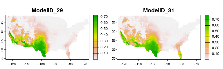
An alternative to strict selection of a single model is to use a consensus model. The main idea is to avoid selecting the best model and instead rely on multiple models with similar performance.
During the prediction of selected models, we calculated model consensus using the mean, median, and a weighted average (using Akaike weights) (Akaike 1973; Wagenmakers and Farrell 2004).
# Consensus projections
plot(preds_E$consensus, mar = c(1, 1, 2, 5))
An important step in understanding the ecological niches with these models is to explore variable response curves. The following lines of code help to do so:
# Response Curves for Bio_1 and Bio_2, first selected model
response_curve(fitted = fits, modelID = "ModelID_29", variable = "bio_1")
response_curve(fitted = fits, modelID = "ModelID_29", variable = "bio_12")

# Consensus Response Curves for Bio_1 and Bio_2, for both models
response_curve(fits, variable = "bio_1")
response_curve(fits, variable = "bio_12")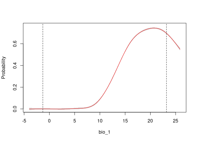

It is useful to examine whether the effect of one variable depends on
the level of other variables. If it does, then we have what is called an
‘interaction’. According to the calibration results from this example,
in both models, the predictor bio_1:bio_12 was selected. To
explore the interaction of these two variables, the function
resp2var can help us to visualize this interaction.
# Consensus Response Curves for Bio_1 and Bio_2, for both models
resp2var(model = fits,
modelID = "ModelID_29",
main = "ModelID 29",
variable1 = "bio_1",
variable2 = "bio_12",
extrapolate = TRUE,
add_limits = TRUE)
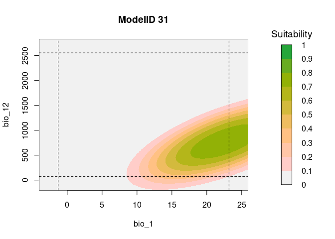
resp2var(model = fits,
modelID = "ModelID_31",
main = "ModelID 31",
variable1 = "bio_1",
variable2 = "bio_12",
extrapolate = TRUE,
add_limits = TRUE)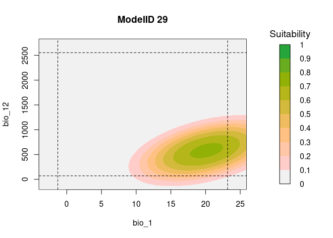
Variable importance or contribution to models can be calculated as a function of the relative deviance explained by each predictor.
Analysis of Deviance for the first selected model:
anova(fits$glms_fitted$ModelID_29, test = "Chi")
#> Analysis of Deviance Table
#>
#> Model: binomial, link: logit
#>
#> Response: Sp
#>
#> Terms added sequentially (first to last)
#>
#>
#>              Df Deviance Resid. Df Resid. Dev  Pr(>Chi)
#> NULL                          5626     3374.9
#> bio_1         1   869.35      5625     2505.6 < 2.2e-16 ***
#> I(bio_1^2)    1    46.77      5624     2458.8 7.972e-12 ***
#> I(bio_12^2)   1   239.69      5623     2219.1 < 2.2e-16 ***
#> bio_1:bio_12  1    42.40      5622     2176.7 7.450e-11 ***
#> ---
#> Signif. codes:  0 '***' 0.001 '**' 0.01 '*' 0.05 '.' 0.1 ' ' 1
Using a function from enmpa you can also explore
variable importance in terms of contribution.
# Relative contribution of the deviance explained for the first model
var_importance(fitted = fits, modelID = "ModelID_29")
#>      predictor contribution cum_contribution
#> 3  I(bio_12^2)    0.3572673        0.3572673
#> 1        bio_1    0.2919587        0.6492259
#> 2   I(bio_1^2)    0.2031750        0.8524009
#> 4 bio_1:bio_12    0.1475991        1.0000000
The function also allows to plot the contributions of the variables for the two models together which can help with the interpretations:
# Relative contribution of the deviance explained
vi_both_models <- var_importance(fits)
# Plot
plot_importance(vi_both_models, extra_info = TRUE)
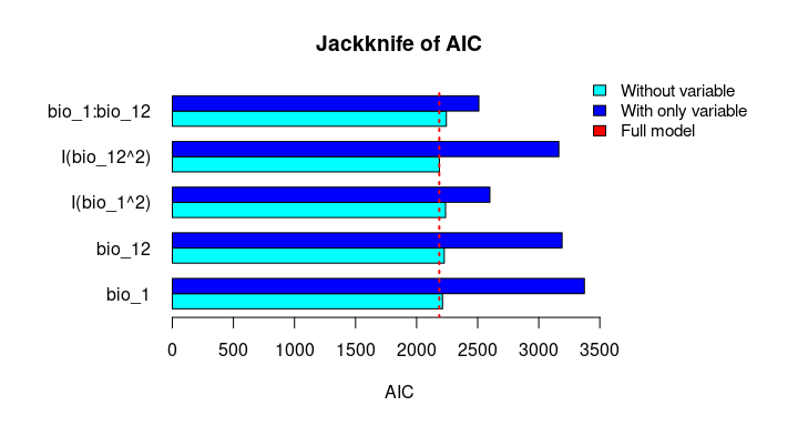
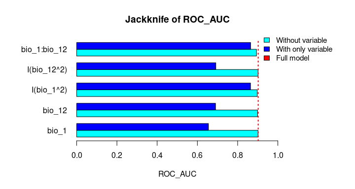
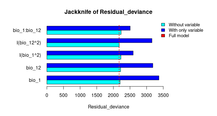
The Jackknife function providing a detailed reflection of the impact of each variable on the overall model, considering four difference measures: ROC-AUC, TSS, AICc, and Deviance.
# Jackknife test
jk <- jackknife(data = enm_data,
          dependent = "Sp",
          independent = c("bio_1", "bio_12"),
          response_type = "lpq")

jk
#> $Full_model_stats
#>     ROC_AUC       TSS     AIC Residual_deviance
#> 1 0.9023279 0.6732916 2185.68           2173.68
#>
#> $Formula
#> [1] "Sp ~ bio_1 + bio_12 + I(bio_1^2) + I(bio_12^2) + bio_1:bio_12"
#>
#> $Without
#>                ROC_AUC       TSS      AIC Residual_deviance
#> bio_1        0.9015319 0.6707435 2212.307          2202.307
#> bio_12       0.8991734 0.6684712 2226.488          2216.488
#> I(bio_1^2)   0.8978504 0.6651925 2237.051          2227.051
#> I(bio_12^2)  0.9016647 0.6744525 2186.700          2176.700
#> bio_1:bio_12 0.8938496 0.6600718 2243.562          2233.562
#>
#> $With_only
#>                ROC_AUC       TSS      AIC Residual_deviance
#> bio_1        0.6549700 0.2970911 3373.978          3369.978
#> bio_12       0.6902666 0.2871473 3191.205          3187.205
#> I(bio_1^2)   0.8641785 0.5786819 2599.638          2595.638
#> I(bio_12^2)  0.6916871 0.2894878 3164.568          3160.568
#> bio_1:bio_12 0.8646620 0.5868336 2509.565          2505.565
# Jackknife plots
plot_jk(jk, metric = "TSS")
plot_jk(jk, metric = "AIC")
plot_jk(jk, metric = "ROC_AUC")
plot_jk(jk, metric = "Residual_deviance")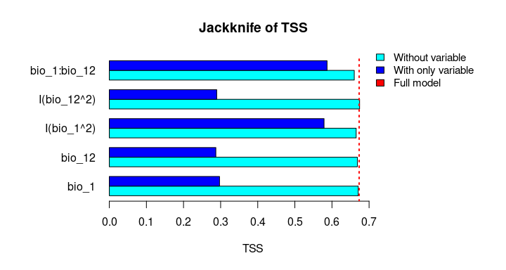
Finally, we will evaluate the final models using the “independent_eval” functions. Ideally, the model should be evaluated with an independent data set (i.e., data that was not used during model calibration or for final model fitting).
# Loading an independent dataset
data("test", package = "enmpa")

# The independent evaluation data are divided into two groups:
# presences-absences (test_01) and presences-only (test_1).
test_1  <- test[test$Sp == 1,]
test_01 <- test

head(test_1)
#>    Sp       lon      lat
#> 4   1 -117.5543 33.62975
#> 8   1 -100.9363 38.68424
#> 19  1 -110.4748 37.78367
#> 53  1 -106.2348 31.70118
#> 54  1 -112.3623 39.35173
#> 60  1 -109.3399 38.26670
head(test_01)
#>   Sp       lon      lat
#> 1  0 -105.6639 35.81247
#> 2  0 -107.9354 33.37200
#> 3  0 -100.3134 48.96018
#> 4  1 -117.5543 33.62975
#> 5  0 -120.6168 36.59670
#> 6  0 -105.3379 40.08928
Using independent data for which presence and absence is known can give the most robust results. Here an example:
projections <- list(
  ModelID_29 = preds_E$predictions$ModelID_29,
  ModelID_31 = preds_E$predictions$ModelID_31,
  Consensus_WA = preds_E$consensus$Weighted_average
)

ie_01 <- lapply(projections, function(x){
  independent_eval01(prediction = x,
                     observation = test_01$Sp,
                     lon_lat = test_01[, c("lon", "lat")])
})

ie_01
#> $ModelID_29
#>     Threshold_criteria Threshold   ROC_AUC False_positive_rate Accuracy
#> 204                ESS 0.1365298 0.9570991          0.08988764     0.91
#> 175             maxTSS 0.1170256 0.9570991          0.10112360     0.91
#> 196              SEN90 0.1311493 0.9570991          0.10112360     0.90
#>     Sensitivity Specificity       TSS
#> 204   0.9090909   0.9101124 0.8192033
#> 175   1.0000000   0.8988764 0.8988764
#> 196   0.9090909   0.8988764 0.8079673
#>
#> $ModelID_31
#>     Threshold_criteria Threshold   ROC_AUC False_positive_rate Accuracy
#> 239                ESS 0.1579818 0.9570991          0.08988764     0.91
#> 205             maxTSS 0.1354130 0.9570991          0.10112360     0.91
#> 218              SEN90 0.1440422 0.9570991          0.10112360     0.90
#>     Sensitivity Specificity       TSS
#> 239   0.9090909   0.9101124 0.8192033
#> 205   1.0000000   0.8988764 0.8988764
#> 218   0.9090909   0.8988764 0.8079673
#>
#> $Consensus_WA
#>     Threshold_criteria Threshold   ROC_AUC False_positive_rate Accuracy
#> 226                ESS 0.1500930 0.9570991          0.08988764     0.91
#> 192             maxTSS 0.1274123 0.9570991          0.10112360     0.91
#> 210              SEN90 0.1394197 0.9570991          0.10112360     0.90
#>     Sensitivity Specificity       TSS
#> 226   0.9090909   0.9101124 0.8192033
#> 192   1.0000000   0.8988764 0.8988764
#> 210 0.9090909 0.8988764 0.8079673When only presence data is available, the evaluation of performance is based on the omission error and the partial ROC analysis.
To do this in our example, we will need to define a threshold value. We can use any of the three threshold values obtained above: ESS, maxTSS or SEN90.
# In this example, we will use the weighted average of the two selected models.

# Consensus_WA
Consensus_WA_T1 <- ie_01[["Consensus_WA"]][1, "Threshold"] # ESS
Consensus_WA_T2 <- ie_01[["Consensus_WA"]][2, "Threshold"] # maxTSS
Consensus_WA_T3 <- ie_01[["Consensus_WA"]][3, "Threshold"] # SEN90

aux_list <- list(ESS = Consensus_WA_T1, maxTSS = Consensus_WA_T2,
                  SEN90 = Consensus_WA_T3)

lapply(aux_list, function(th){
  independent_eval1(prediction = projections[["Consensus_WA"]],
                    threshold = th,
                    lon_lat = test_1[, c("lon", "lat")])

})
#> $ESS
#>   omission_error threshold Mean_AUC_ratio pval_pROC
#> 1     0.09090909  0.150093       1.634595         0
#>
#> $maxTSS
#>   omission_error threshold Mean_AUC_ratio pval_pROC
#> 1              0 0.1274123        1.63588         0
#>
#> $SEN90
#>   omission_error threshold Mean_AUC_ratio pval_pROC
#> 1     0.09090909 0.1394197       1.632866         0