![]()
The hemispheR package allows processing digital hemispherical
(also called fisheye) images (either circular or fullframe) of forest
canopies to retrieve canopy attributes like canopy
openness and leaf area index (LAI).
You can install hemispheR from CRAN:
install.packages('hemispheR')You can install the development version of hemispheR
using devtools:
# install.packages("devtools")
devtools::install_git("https://gitlab.com/fchianucci/hemispheR")A distinct feature of (circular) hemispherical images is that a circular mask should be applied to exclude outer pixels from analyses.
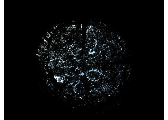
The import_fisheye() function allows importing fisheye
images as:
img<-import_fisheye(image,
                    channel = 3,
                    circ.mask=list(xc=1136,yc=852,rc=754),
                    circular=TRUE,
                    gamma=2.2,
                    stretch=FALSE,
                    display=TRUE,
                    message=TRUE)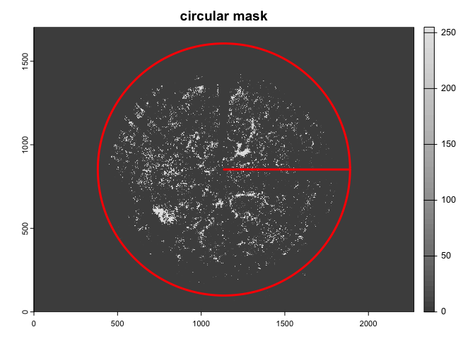
The function has the following parameters:
- filename: the input image name; any kind of image (i.e.,
raster matrix) can be read using terra::rast()
functionality;
- channel: the band number (Default value is 3, corresponding
to blue channel in RGB images, which can be equivalently selected as
‘B’). Mixing channel options are also available such as ‘GLA’, ‘Luma’,
‘2BG’, ‘GEI’, ‘RGB’, see explanations later;
- circ.mask: a list of three-parameters (x-center (xc),
y-center (yc), radius (rc)) needed to apply a circular mask. These
parameters can be also derived using the camera_fisheye()
function for known camera+lenses. If missing, they are automatically
calculated;
- circular: it allows to specify if the fisheye image is
circular (circular=TRUE) or fullframe (circular=FALSE)
type; it affects the way the radius (rc) is calculated in case
circ.mask is omitted;
- gamma: the actual gamma of the image, which is then
back-corrected. Default value is 2.2, as typical of most image formats
(e.g. jpeg images). If no gamma correction is required, just write
gamma=1;
- stretch: optionally, users can decide to apply a linear
stretch to the select image channel, to enhance contrast;
- display: if TRUE, a plot of the imported image is displayed
along with the circular mask applied;
- message: if TRUE, a message about the mask parameters applied
to image is printed.
For circular mask, there is an utility function
camera_fisheye() which provides the three-parameters for a
long list of camera+fisheye equipments, which can be screened by typing
list.cameras as in the example below:
list.cameras
#>  [1] "Coolpix950+FC-E8"  "Coolpix990+FC-E8"  "Coolpix995+FC-E8"
#>  [4] "Coolpix4500+FC-E8" "Coolpix5000+FC-E8" "Coolpix5400+FC-E9"
#>  [7] "Coolpix8700+FC-E9" "Coolpix8400+FC-E9" "Coolpix8800+FC-E8"
#> [10] "D60+Sigma-4.5"     "D80+Sigma-4.5"     "D90+Sigma-4.5"
#> [13] "D300+Sigma-4.5"    "EOS300+Regent-4.9" "EOS20D+Sigma-4.5"
#> [16] "EOS30D+Sigma-4.5"  "EOSXSi+Sigma-4.5"  "EOST1i+Sigma-4.5"
#> [19] "EOST2i+Sigma-4.5"  "EOST3i+Sigma-4.5"
Using the camera_fisheye(), the importing will be:
img<-import_fisheye(image,
                    circ.mask=camera_fisheye('Coolpix4500+FC-E8'))
The import_fisheye() function can also import fullframe
fisheye images, by setting circular=FALSE:
img2<-import_fisheye(image2,
               circular=FALSE,
               gamma=2.2,
               display=TRUE,
               message=TRUE)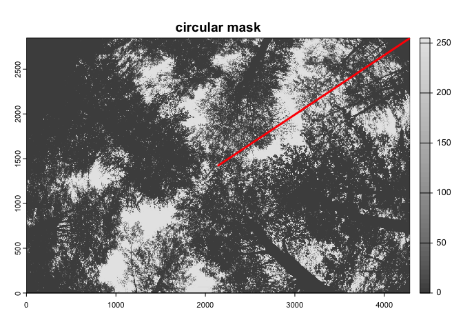
Beside the numeric bands, other options in the channel
argument are:
\[ GEI=2G-R-B \]
\[ GLA=\frac{2G-R-B}{2G+R+B} \]
\[ Luma=0.3R+0.59G+0.11B \]
\[ RGB=\frac{R+G+B}{3} \]
\[ 2BG=2B-G \]
Both the Green Excess Index (‘GEI’) and the Green Leaf Algorithm (‘GLA’) are visible (RGB) vegetation indexes, which are often used for short canopies or downward-looking images (see also below). The’Luma’ method provides a weighted mean of RGB linear components, which resembles human’s colors perception (HSP color model). The ‘2BG’ method aimed to enhance contrast between canopy and sky pixels by lightening the blue and darkening the green.
Note: you can also process images hemispherical image created from smartphone panorama images. A tool is described here: https://www.azandisresearch.com/2023/05/20/update-smartphone-hemispherical-image-analysis/.
Once imported, the function performs image classification using a
single automated thresholding from the auto_thresh()
functionality of the autothresholdr
package:
img.bw<-binarize_fisheye(img,
                         method='Otsu',
                         zonal=FALSE,
                         manual=NULL,
                         display=TRUE,
                         export=FALSE)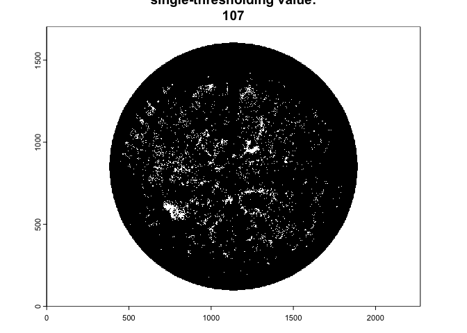
Where:
- img: is the input single-channel raster generated from
import_fisheye();
- method: is the automated thresholding method. Default is set
to ‘Otsu’; for For other methods, see: https://imagej.net/plugins/auto-threshold;
- zonal: if set to TRUE, it divides the image in four sectors
(NE,SE,SW,NW directions) and applies an automated classification
separatedly to each region; useful in case of uneven light conditions in
the image;
- manual: alternatively to the automated method, users can
insert a numeric threshold value; in this case, manual thresholding
overrides automated classification;
- display: if set to TRUE, a plot of the classified image is
displayed;
- export: if set tot TRUE, a binary jpeg image is stored in a
“result” folder.
As the import_fisheye() function also allows to
calculate grenness indices, the package could be also used for importing
and classifying downward-looking fisheye images:
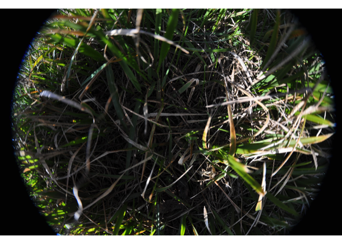
In such a case, we suggest to use the thresholding method=‘Percentile’ in combination with a grenness index:
downimg |>
  import_fisheye(channel='GLA',circ.mask=list(xc=2144,yc=1424,rc=2050),stretch=TRUE) |>
binarize_fisheye(method='Percentile',display=TRUE) 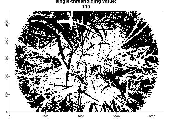
#> class : SpatRaster
#> dimensions : 2848, 4288, 1 (nrow, ncol, nlyr)
#> resolution : 1, 1 (x, y)
#> extent : 0, 4288, 0, 2848 (xmin, xmax, ymin, ymax)
#> coord. ref. :
#> source(s) : memory
#> varname : circular_downward_D90-8-15
#> name : circular_downward_D90-8-15.jpg
#> min value : 0
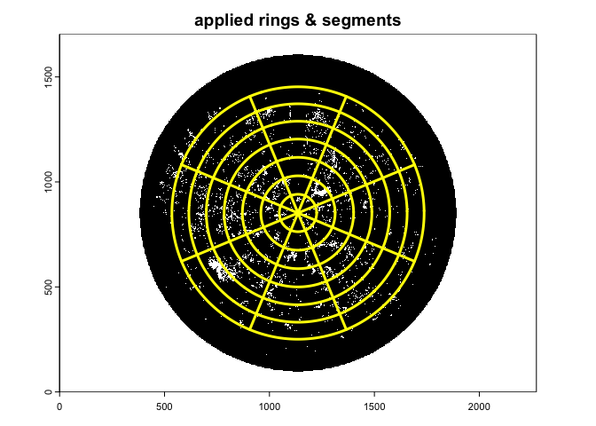
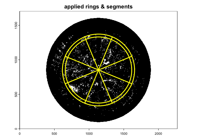
#> max value : 1The gapfrac_fisheye() function retrieve the angular
distribution from classified fisheye images, considering the fisheye
lens correction, as:
gap.frac<-gapfrac_fisheye(
  img.bw,
  maxVZA = 90,
  lens = "FC-E8",
  startVZA = 0,
  endVZA = 70,
  nrings = 7,
  nseg = 8,
  display=TRUE,
  message = FALSE
)
head(gap.frac)
#>                                        id ring     GF0_45    GF45_90   GF90_135
#> 1 circular_coolpix4500+FC-E8_chestnut.jpg    5 0.03561298 0.07041801 0.04254649
#> 2 circular_coolpix4500+FC-E8_chestnut.jpg   15 0.06794124 0.04197934 0.20285159
#> 3 circular_coolpix4500+FC-E8_chestnut.jpg   25 0.10305717 0.06669285 0.08786911
#> 4 circular_coolpix4500+FC-E8_chestnut.jpg   35 0.08239523 0.04155401 0.05836723
#> 5 circular_coolpix4500+FC-E8_chestnut.jpg   45 0.02757889 0.03303338 0.03144297
#> 6 circular_coolpix4500+FC-E8_chestnut.jpg   55 0.06891697 0.01458520 0.01906895
#>    GF135_180  GF180_225  GF225_270  GF270_315   GF315_360  lens         circ
#> 1 0.12668810 0.05609833 0.04019293 0.06649858 0.006752412 FC-E8 1136_852_754
#> 2 0.14235998 0.11460359 0.12028276 0.04903867 0.056008700 FC-E8 1136_852_754
#> 3 0.07853917 0.05599374 0.09634138 0.06792256 0.106224229 FC-E8 1136_852_754
#> 4 0.10967222 0.03381894 0.08813624 0.11716016 0.061097671 FC-E8 1136_852_754
#> 5 0.05687816 0.01977497 0.06933212 0.11588438 0.073508752 FC-E8 1136_852_754
#> 6 0.05737915 0.08741001 0.07077830 0.19257719 0.036927811 FC-E8 1136_852_754
#>   channel stretch gamma zonal thd method
#> 1       3   FALSE   2.2 FALSE 107   Otsu
#> 2       3   FALSE   2.2 FALSE 107   Otsu
#> 3       3   FALSE   2.2 FALSE 107   Otsu
#> 4       3   FALSE   2.2 FALSE 107   Otsu
#> 5       3   FALSE   2.2 FALSE 107   Otsu
#> 6       3   FALSE   2.2 FALSE 107   Otsu
where:
- img.bw: is the input single-channel binary image generated
from binarize_fisheye();
- maxVZA: is the maximum zenith angle (degree) corresponding to
the radius; it is used to perform lens correction. Default value is set
to 90;
- startVZA: is the lower zenith angle (degree) used for
analysis. Default values is set to 0;
- endVZA: is the upper zenith angle (degree) used for analysis.
Default value is set to 70;
- lens: define the lens type used for correcting fisheye
distortion; see list.lenses for a list of various fisheye
lens available. If omitted, an equidistant projection is assumed by
default;
- nrings: number of zenith rings;
- nseg: number of azimuth sectors;
- display: if set to TRUE, it overlaids the image with the
zenith and azimuth bins;
- message: if set to TRUE, it reports the applied mask used in
the analysis.
A suggested setting for comparability with LAI-2000/2200 Plant Canopy Analyzer (five rings, each about 15 degrees in size) is:
gap.frac2<-gapfrac_fisheye(
  img.bw,
  maxVZA = 90,
  lens = "FC-E8",
  startVZA = 0,
  endVZA = 75,
  nrings = 5,
  nseg = 8,
  display=TRUE,
  message = FALSE
)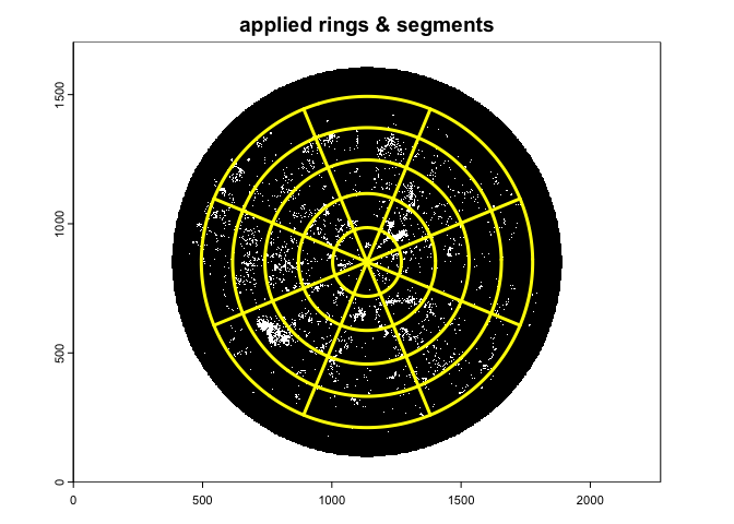
With this setting the Le is comparable with the apparent L derived from LAI-2000/2200 (see Chianucci et al. 2015).
A suggested setting for implementing the hinge angle method (Bonhomme and Chartier 1972), which uses a fixed restricted view angle centered at 1 radian - about 57 degree, is:
gap.frac3<-gapfrac_fisheye(
  img.bw,
  maxVZA = 90,
  lens = "FC-E8",
  startVZA = 55,
  endVZA = 60,
  nrings = 1,
  nseg = 8,
  display=TRUE,
  message = FALSE
)
A long list of projection functions is available for the
lens argument, which can be screened by typing:
list.lenses
#>  [1] "equidistant"             "orthographic"
#>  [3] "stereographic"           "equisolid"
#>  [5] "Aico-ACHIR01028B10M"     "Aico-ACHIR01420B9M"
#>  [7] "ArduCam-M25156H18"       "Bosch-Flexidome-7000"
#>  [9] "Canon-RF-5.2"            "CanonEF-8-15"
#> [11] "DZO-VRCA"                "Entaniya-HAL-200"
#> [13] "Entaniya-HAL-250"        "Entaniya-M12-220"
#> [15] "Entaniya-M12-250"        "Entaniya-M12-280"
#> [17] "Evetar-E3267A"           "Evetar-E3279"
#> [19] "Evetar-E3307"            "FC-E8"
#> [21] "FC-E9"                   "iZugar-MKX13"
#> [23] "iZugar-MKX19"            "iZugar-MKX200"
#> [25] "iZugar-MKX22"            "Kodak-SP360"
#> [27] "Laowa-4"                 "Lensagon-BF10M14522S118"
#> [29] "Lensagon-BF16M220D"      "Meike-3.5"
#> [31] "Meike-6.5"               "Nikkor-10.5"
#> [33] "Nikkor-8"                "Nikkor-OP10"
#> [35] "Omnitech-ORIFL190-3"     "Raynox-CF185"
#> [37] "Sigma-4.5"               "Sigma-8"
#> [39] "SMTEC-SL-190"            "Soligor"
#> [41] "Sunex-DSL239"            "Sunex-DSL315"
#> [43] "Sunex-DSL415" "Sunex-DSLR01"The canopy_fisheye() function inverts angular gap
fraction from fisheye images to derive forest canopy attributes. The
function allows to estimate both effective (Le) and actual
(L) Leaf area index (LAI) using the Miller’s (1967)
theorem:
\[ LAI =2 \int_{0}^{\pi/2} -ln[P_0(\theta)] cos\theta \sin \theta d \theta \]
Effective (Le) or actual (L) LAI is calculated from the formula depending on whether the logarithm of the arithmetic \(ln(\overline{P_0(\theta)}\) or geometric \(\overline{ln(P_0(\theta))}\) mean \(P_0(\theta)\) is considered (see explanation in Chianucci et al. 2019. The \(cos\theta d\theta\) is normalized to sum as unity.
Please note that for leaf area inversion, the function replace empty gaps (where gap fraction is zero) with a fixed value set to 0.00004530 (which corresponds to a saturated LAI value of 10) as the logarithm of zero gap fraction is not defined.
Different clumping indices are derived from the
canopy_fisheye() function. The Lang & Xiang
(1986) (LX) is calculated as the ratio of Le to L derived from the
Miller theorem.
Two clumping indices (LXG) were derived from an ordered weighted average (OWA) gap fraction (see Chianucci et al. 2019):
\[ \Omega_{LXG}= \frac {-\int_{0}^{\pi/2}ln[\sum_{i=1}^{n}w_i^{'}P_{i\downarrow}\theta]cos\theta d\theta}{{-\int_{0}^{\pi/2}ln[\sum_{i=1}^{n}w_i^{'}P_{i\uparrow}\theta}]cos\theta d\theta} \]
where w’ is a normalized, non-increasing weighting vector. The \(cos\theta d\theta\) is normalized to sum as unity.
Two weighting vectors are applied:
\[ w_i^{'}=\frac{2(n+1-i)}{n(n+1)} \]
for \(\Omega_{LXG1}\) and
\[ w_i^{'}= \frac{1}{n}\sum_{j=1}^{n}\frac{1}{j} \]
for \(\Omega_{LXG2}\).
The LXG considers both the gap fraction distribution as in LX, and the gap magnitude, resulting in higher clumping correction than LX. For details, see Chianucci et al. 2019).
Diffuse non-interceptance (DIFN) also called canopy openness is calculated as the mean gap fraction weighted for the ring area, as reported in the LAI-2200 manual (Li-Cor Inc., Nebraska US), (Equation 10-25). Unlike LAI-2200 however, DIFN is calculated from the arithmetic mean gap fraction of each ring.
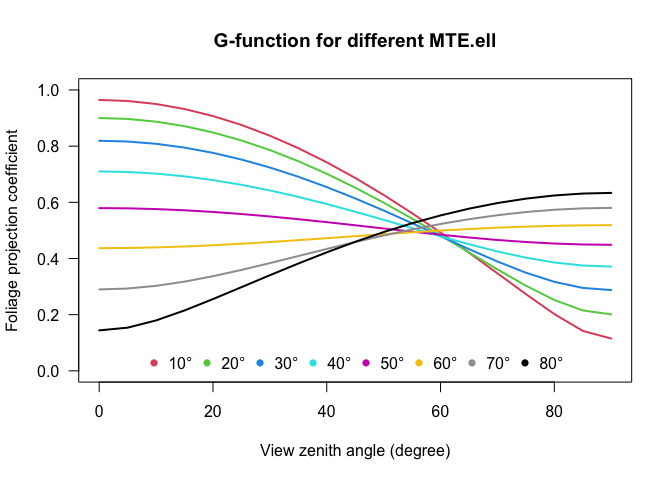
Additional variables are the mean leaf tilt angle (MTA.ell), which is calculated from the original formula by Norman and Campbell (1989) using an Ellipsoidal distribution with one-parameter x. The ellipsoidal extinction coefficient is given by:
\[ k(\theta,x)=\frac{\sqrt{x^{2}+tan^{2}(\theta)}}{x+1.702(x+1.12)^{-0.708}} \]
and
\[ MTA.ell=90\times{(0.1+0.9e^{-0.5x})} \]
From the Ellipsoidal distribution function it is also possible to calculate the Foliage projection function (G-function; \(G(\theta)=k(\theta,x)\times cos(\theta)\) based on the MTA.ell:
All these algorithms are applied by simply typing:
canopy<-canopy_fisheye(gap.frac2)
canopy
#> # A tibble: 1 × 20
#>   id         Le     L    LX  LXG1  LXG2  DIFN MTA.ell     x VZA   rings azimuths
#>   <chr>   <dbl> <dbl> <dbl> <dbl> <dbl> <dbl>   <dbl> <dbl> <chr> <int>    <int>
#> 1 circul…  3.65  3.86  0.95  0.84  0.76  6.19      36  2.21 7.5_…     5        8
#> # ℹ 8 more variables: mask <chr>, lens <chr>, channel <chr>, stretch <chr>,
#> # gamma <chr>, zonal <chr>, method <chr>, thd <chr>Arietta, A.A., 2022. Estimation of forest canopy structure and understory light using spherical panorama images from smartphone photography. Forestry, 95(1), pp.38-48. https://doi.org/10.1093/forestry/cpab034
Bonhomme, R. and Chartier, P., 1972. The interpretation and automatic measurement of hemispherical photographs to obtain sunlit foliage area and gap frequency. Israel Journal of Agricultural Research, 22, pp.53-61.
Campbell, G.S., 1986. Extinction coefficients for radiation in plant canopies calculated using an ellipsoidal inclination angle distribution. Agricultural and forest meteorology, 36(4), pp.317-321. https://doi.org/10.1016/0168-1923(86)90010-9
Chianucci, F., Macfarlane, C., Pisek, J., Cutini, A. and Casa, R., 2015. Estimation of foliage clumping from the LAI-2000 Plant Canopy Analyzer: effect of view caps. Trees, 29(2), pp.355-366. https://doi.org/10.1007/s00468-014-1115-x
Chianucci, F., Zou, J., Leng, P., Zhuang, Y. and Ferrara, C., 2019. A new method to estimate clumping index integrating gap fraction averaging with the analysis of gap size distribution. Canadian Journal of Forest Research, 49(5), pp.471-479. https://doi.org/10.1139/cjfr-2018-0213
Chianucci, F. and Macek, M., 2023. hemispheR: an R package for fisheye canopy image analysis. Agricultural and Forest Meteorology, 336, p.109470. https://doi.org/10.1016/j.agrformet.2023.109470
Landini, G., Randell, D.A., Fouad, S. and Galton, A., 2017. Automatic thresholding from the gradients of region boundaries. Journal of microscopy, 265(2), pp.185-195. https://doi.org/10.1111/jmi.12474
Lang, A.R.G. and Xiang, Y., 1986. Estimation of leaf area index from transmission of direct sunlight in discontinuous canopies. Agricultural and forest Meteorology, 37(3), pp.229-243. https://doi.org/10.1016/0168-1923(86)90033-X
Louhaichi, M., Borman, M.M. and Johnson, D.E., 2001. Spatially located platform and aerial photography for documentation of grazing impacts on wheat. Geocarto International, 16(1), pp.65-70. https://doi.org/10.1080/10106040108542184
Miller, J.B. A formula for average foliage density. Australian Journal of Botany, 15 (1967), pp. 141-144
Norman, J.M. and Campbell, G.S., 1989. Canopy structure. In Plant physiological ecology: field methods and instrumentation (pp. 301-325). Dordrecht: Springer Netherlands. https://doi.org/10.1007/978-94-009-2221-1_14