
The R package easybgm provides a
user-friendly package for performing a Bayesian analysis of psychometric
networks. In particular, it helps to fit, extract, and visualize the
results of a Bayesian graphical model commonly used in the social and
behavioral sciences. The package is a wrapper around existing packages.
So far, the package supports fitting and extracting results of
cross-sectional network models using BDgraph (Mohammadi
& Wit, 2015), BGGM(Williams & Mulder, 2019), and
bgms (Marsman, van den Bergh & Haslbeck, 2025). As
output, the package extracts the posterior parameter estimates, the
posterior inclusion probability, the inclusion Bayes factor, and
optionally posterior samples of the parameters and the nodes centrality.
The package comes with an extensive suite of visualization functions.
The package now also supports comparing networks across groups. This is
done through Bayesian inference to quantify differences in conditional
(in)dependence structures, using functionality from BGGM
(Williams et al., 2020) and bgms (Marsman et al., 2025). In
addition, it allows users to incorporate clustering assumptions by
specifying a stochastic block prior on the network structure and to test
hypotheses about the presence of such clustering (Sekulovski et al.,
2025) via bgms.
To install this package from Github use
install.packages("remotes")
remotes::install_github("KarolineHuth/easybgm")
To rather install the most up-to-date developer version, use
install.packages("remotes")
remotes::install_github("KarolineHuth/easybgm", ref = "developer")The package consists of wrapper functions around existing R packages
(i.e., BDgraph, bgms, and BGGM).
To initiate estimation, researchers must specify the data set and the
data type (i.e., continuous, mixed, ordinal, or binary). Based on the
data type specification, easybgm estimates the network
using the appropriate R package (i.e., BDgraph for
continuous and mixed data, and bgms for ordinal and binary
data). Users can override the default package selection by specifying
their preferred R package with the package argument. All
other arguments, such as package-specific informed prior specifications,
can be passed to easybgm. As output, easybgm
returns the posterior parameter estimates, the posterior inclusion
probability, and the inclusion Bayes factor. In addition, the package
extracts the posterior samples of the parameters by setting
save = TRUE and the strength centrality samples by setting
centrality = TRUE. When
edge_prior = "Stochastic-Block" is used with
bgms, the output additionally includes the posterior
estimates of node- cluster memberships, the posterior inclusion
probabilities for all possible numbers of clusters, and the posterior
coclustering matrix which depicts the proportion of times each pair of
nodes appeared in the same cluster.
The package comes with an extensive suite of functions to visualize
the results of the Bayesian analysis of networks. We provide more
information on each of the plots below. The visualization functions use
qgraph (Epskamp et al., 2012) or ggplot2
(Wickham, 2016) as the backbone.
The edge evidence plot aids researchers in deciding which edges provide robust inferential conclusions. In the edge evidence plot, edges represent the inclusion Bayes factor \(`\text{BF}_{10}`\). Yellow edges indicate evidence for edge absence (i.e., conditional independence), grey edges indicate the absence of evidence, and blue edges indicate evidence for edge presence (i.e., conditional dependence). Blue edges represent evidence for inclusion, light blue, dashed edges represent weak evidence for inclusion, grey edges represent absence of evidence, light yellow, dashed edges represent some evidence for exclusion, and dark yellow edges represent strong evidence for exclusion. By default, a \(`\text{BF}_{10} > 10`\) is considered strong evidence for inclusion and \(`\text{BF}_{01} > 10`\) for exclusion, and a \(`\text{BF}_{10} > 3`\) is considered weak evidence for inclusion and \(`\text{BF}_{01} > 3`\) for exclusion. Users can specify the threshold for Bayes factors.
In the network plot, edges indicate the strength of partial association between two nodes. The network plot shows all edges with an inclusion Bayes factor greater than \(1\), i.e. all edges that have some evidence of inclusion. Edge thickness and saturation represent the strength of the association; the thicker the edge, the stronger the association. Red edges indicate negative associations and blue edges indicate positive associations.
The structure uncertainty can be assessed with the posterior structure probability plot and the posterior complexity plot. The posterior structure probability plot shows the posterior probabilities of the visited structures, sorted from the most to the least probable. Each dot represents one structure. The more structures with similar posterior probability, the more uncertain the true structure. If one structure dominates the posterior structure probability, we can be relatively certain about the true structure.
The posterior complexity plot shows the posterior probability of a structure complexity (i.e., number of present edges in a network). Here, the posterior probability of all structures with the same complexity are aggregated into one plot.
The 95 % highest density intervals (HDI) of the parameters are visualized with a parameter forest plot. In the plot, dots represent the median of the posterior samples and the lines indicate the shortest interval that covers 95% of the posterior distribution. The narrower an interval, the more stable a parameter.
Researchers often use centrality measures to obtain aggregated information for each node, such as the connectedness quantified by strength centrality. Credible intervals for strength centrality can be obtained by calculating the centrality measure for each sample of the posterior distribution. The higher the centrality, the more connected the node; error bars represent the 95% High Density Interval (HDI).
We want to illustrate the package use with an example. In particular,
we use the women and mathematics data which can be loaded with the
package BGGM. We fit the model and extract its results with
the function easybgm. We specify the data and the data
type, which in this case is binary.
library(easybgm)
library(BGGM)

data <- na.omit(women_math)
colnames(data) <- c("LCA", "GND", "SCT", "NMF", "SBP", "FTP")

res <- easybgm(data, type = "binary")
Having fitted the model, we can now take a look at its results.
summary(res)

#>  BAYESIAN ANALYSIS OF NETWORKS
#>  Model type: binary
#>  Number of nodes: 6
#>  Fitting Package: bgms
#> ---
#>  EDGE SPECIFIC OVERVIEW
#>  Relation Estimate Posterior Incl. Prob. Inclusion BF Category
#>   LCA-GND    0.000                 0.034        0.035 excluded
#>   LCA-SCT    0.001                 0.027        0.028 excluded
#>   GND-SCT    0.003                 0.043        0.044 excluded
#>   LCA-NMF    0.001                 0.038        0.040 excluded
#>   GND-NMF    0.508                 1.000          Inf included
#>   SCT-NMF   -0.012                 0.084        0.092 excluded
#>   LCA-SBP    0.001                 0.031        0.032 excluded
#>   GND-SBP   -0.756                 1.000          Inf included
#>   SCT-SBP    0.337                 0.982       54.556 included
#>   NMF-SBP   -0.980                 1.000          Inf included
#>   LCA-FTP   -0.004                 0.051        0.054 excluded
#>   GND-FTP    0.000                 0.040        0.042 excluded
#>   SCT-FTP    1.176                 1.000          Inf included
#>   NMF-FTP    0.670                 1.000          Inf included
#>   SBP-FTP   -0.014                 0.090        0.099 excluded
#>
#> Bayes Factors larger than 10 were considered sufficient evidence for the categorization.
#>  ---
#>  AGGREGATED EDGE OVERVIEW
#>  Number of included edges: 6
#>  Number of inconclusive edges: 0
#>  Number of excluded edges: 9
#>  Number of possible edges: 15
#>
#>  ---
#>  STRUCTURE OVERVIEW
#>  Number of visited structures: 109
#>  Number of possible structures: 32768
#>  Posterior probability of most likely structure: 0.6264
#> ---
Furthermore, we can visualize the results with plots. In a first
step, we assess the edge evidence plot in which edges represent the
inclusion Bayes factor \(`\text{BF}_{10}`\). In the plot, blue edges
represent evidence for inclusion (default values: \(`\text{BF}_{10} > 10`\)), light blue,
dashed edges represent weak evidence for inclusion (\(`3 < \text{BF}_{10} < 10`\)), grey
edges represent absence of evidence (\(`1/3
< \text{BF}_{10} < 3`\)), light yellow, dashed edges
represent some evidence for exclusion (\(`1/10
< \text{BF}_{10} < 1/3`\)), and dark yellow edges represent
strong evidence for exclusion (\(`\text{BF}_{10} < 1/10`\)). Especially
in a large network, it can be useful to split the edge evidence plot in
two parts by setting the split argument to
TRUE, which splits the plot into the edges with some
evidence for inclusion (i.e., \(`\text{BF}_{10} > 1`\)) and those with
some evidence for exclusion (i.e., \(`\text{BF}_{10} < 1`\)).
plot_edgeevidence(res, edge.width = 2, split = F, legend = F)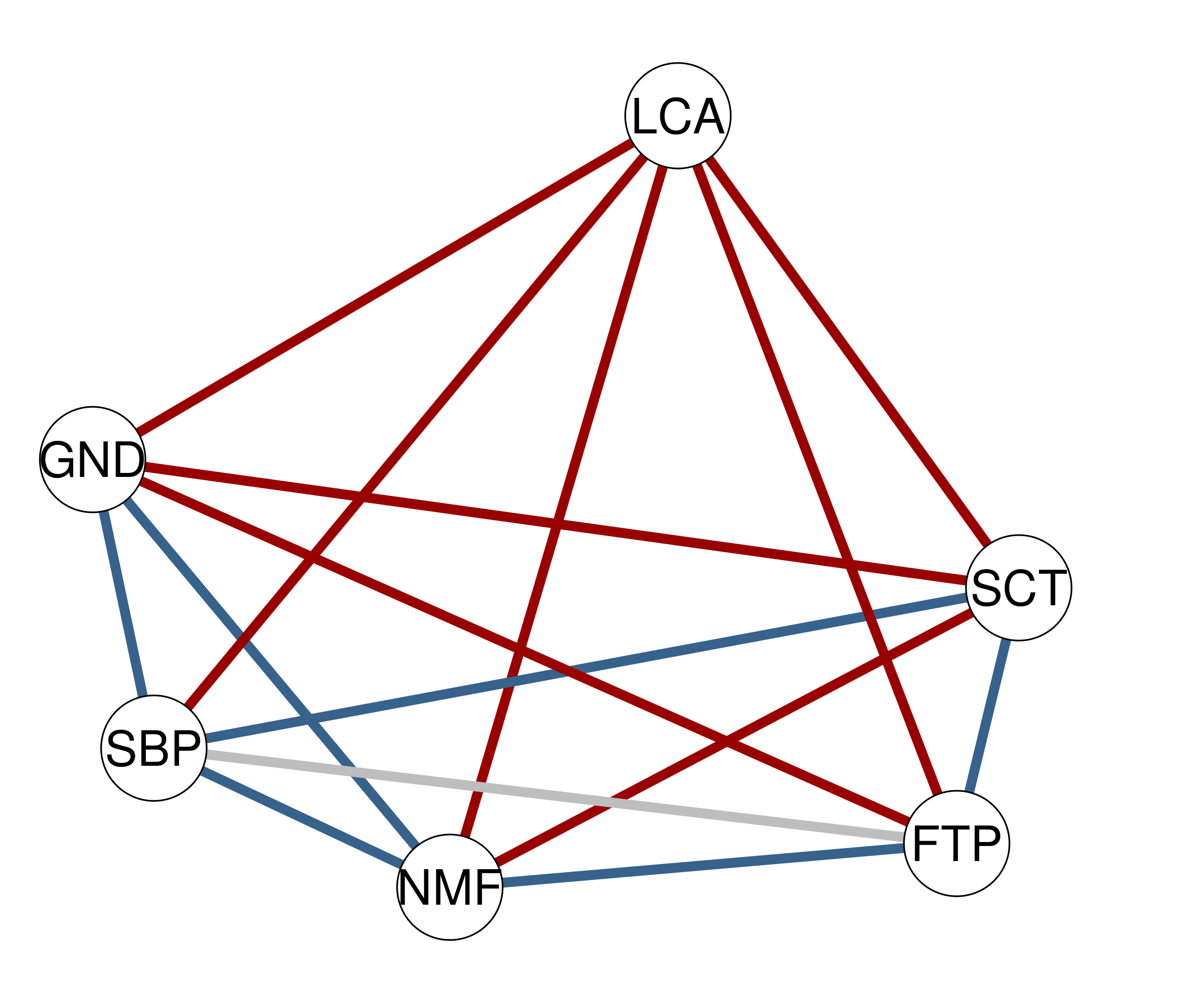
Furthermore, we can look at the network plot in which edges represent the partial associations.
plot_network(res, layout = "spring",
             layoutScale = c(.8,1), palette = "R",
             theme = "TeamFortress", vsize = 6)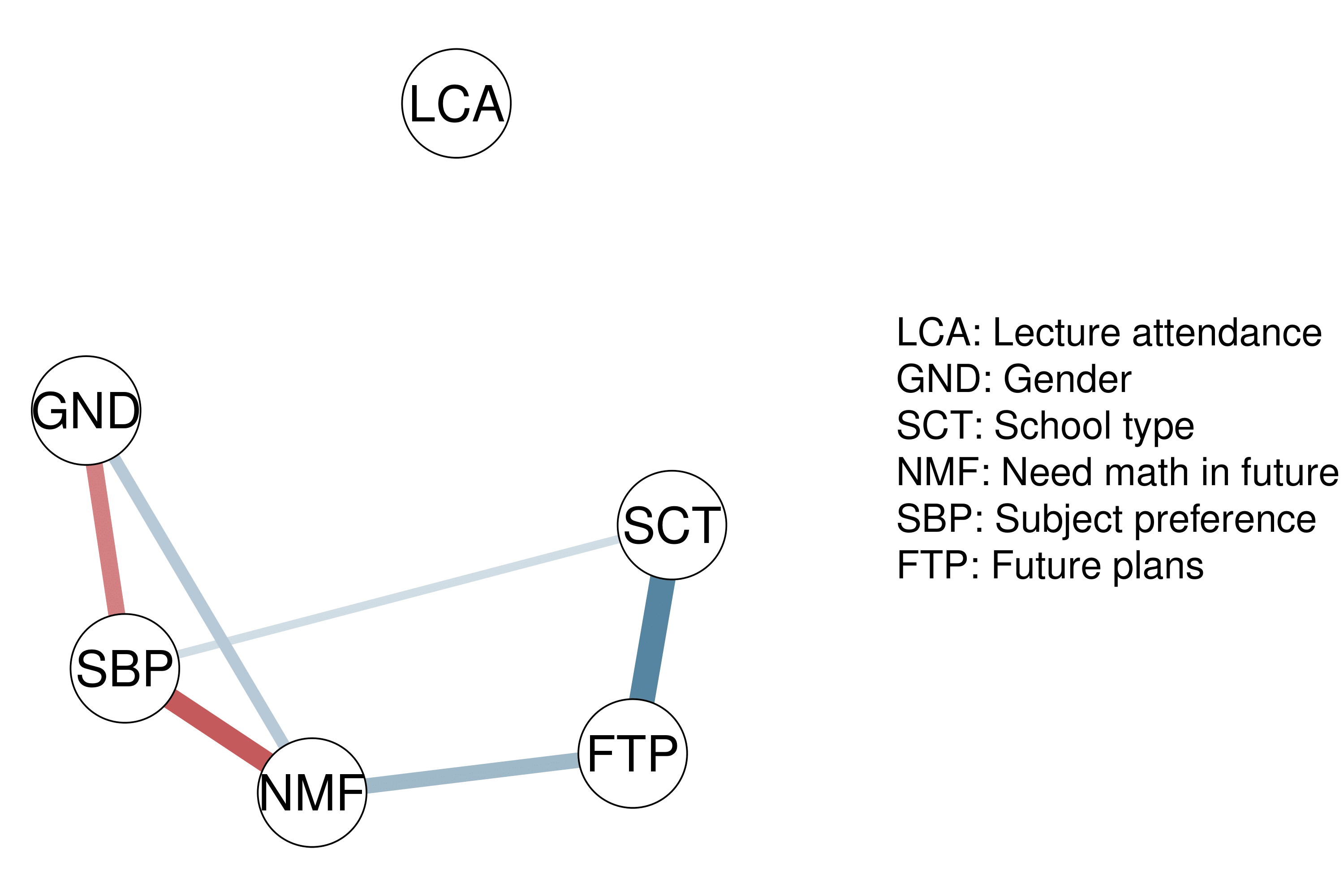
We can also assess the structure specifically with three plots. Note
that this only works, if we use either the BDgraph or
bgms package.
plot_structure_probabilities(res, as_BF = FALSE)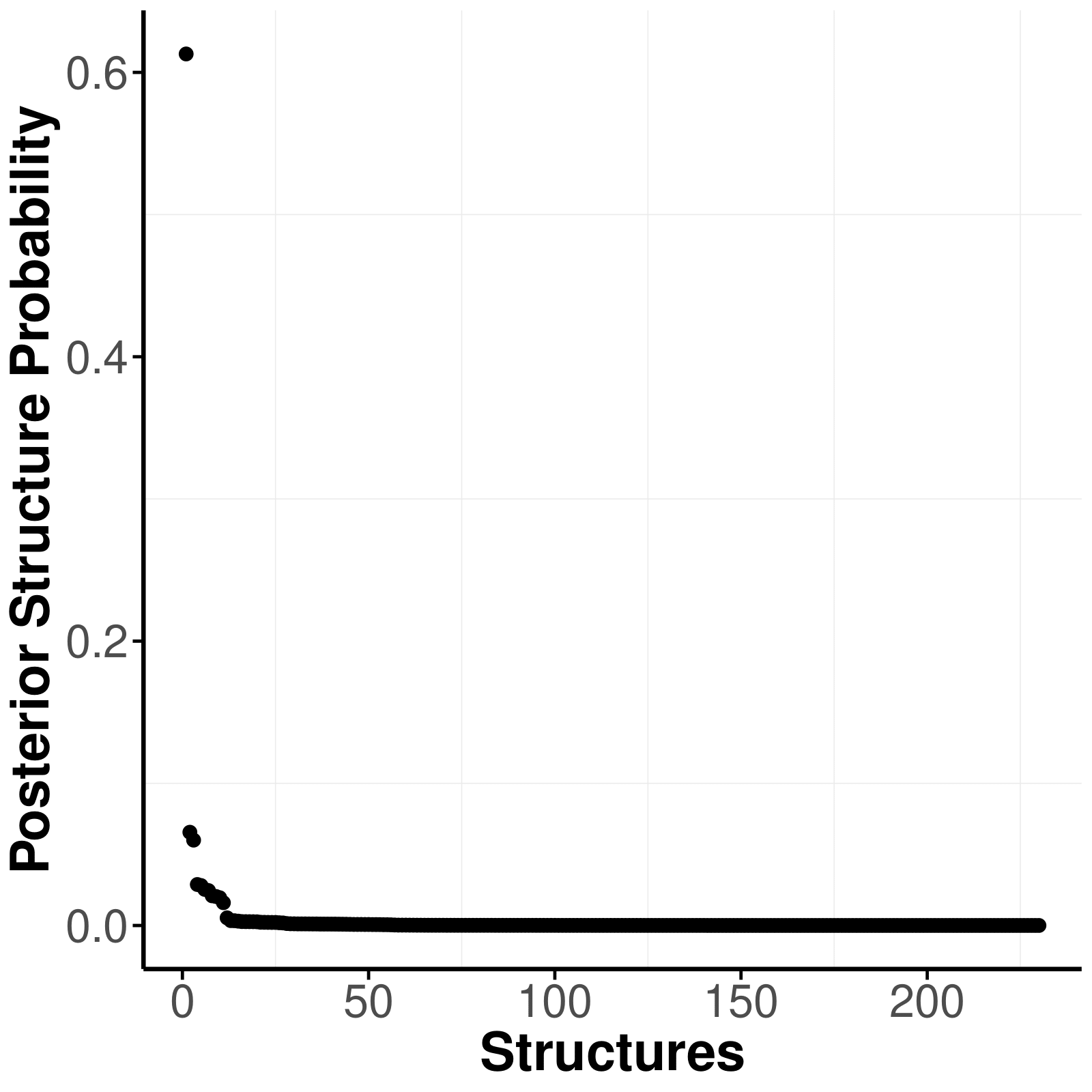
plot_complexity_probabilities(res, as_BF = FALSE)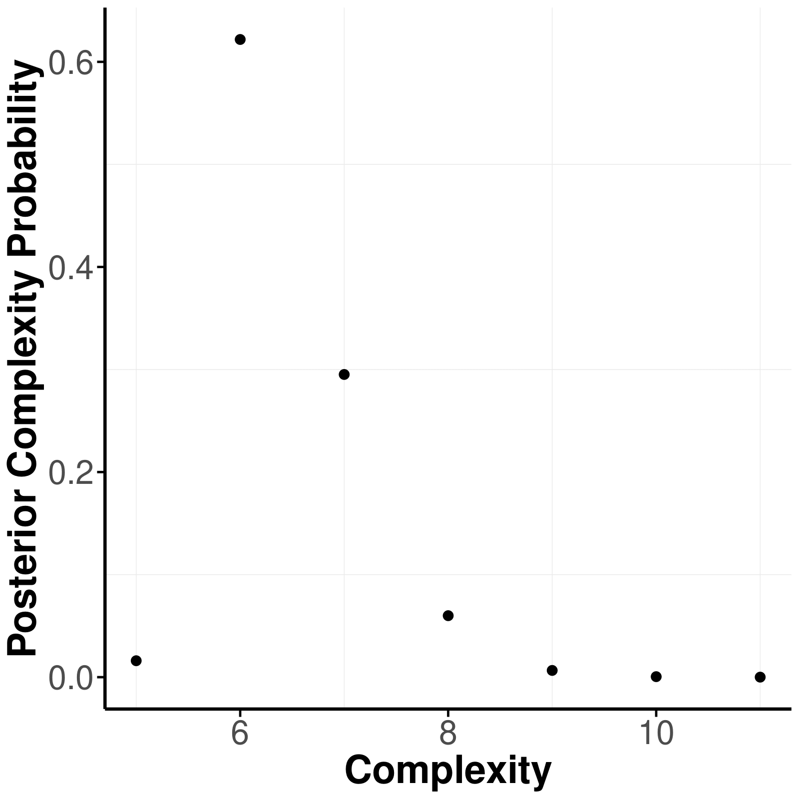
plot_structure(res, layoutScale = c(.8,1), palette = "R",
               theme = "TeamFortress", vsize = 6, edge.width = .3, layout = "spring")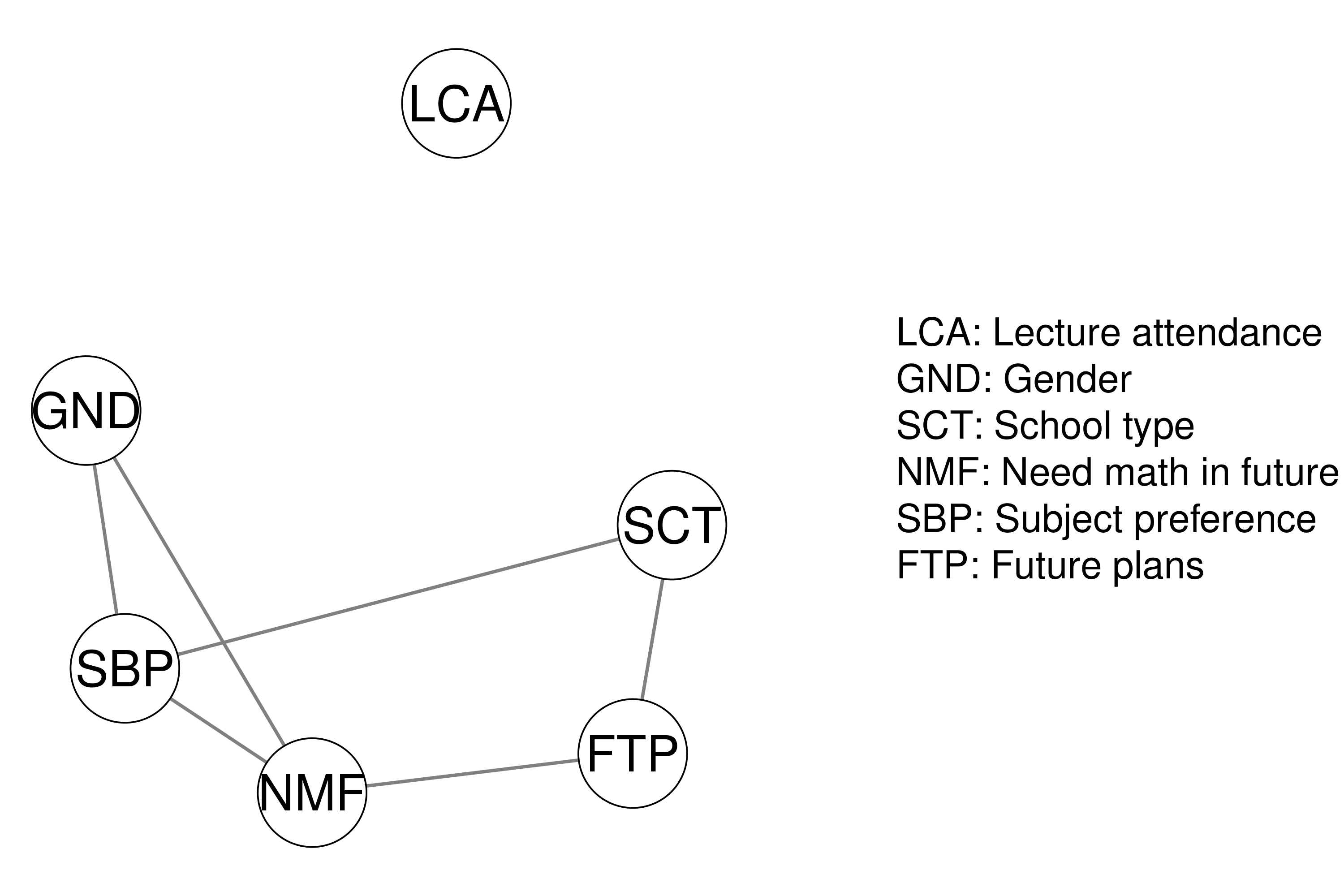
In addition we can obtain posterior samples from the posterior
distribution by setting save = TRUE in the
easybgm function and thereby open up new possibilities of
assessing the model. We can extract the posterior density of the
parameters with a parameter forest plot.
res <- easybgm(data, type = "binary", save = TRUE, centrality = TRUE)
plot_parameterHDI(res)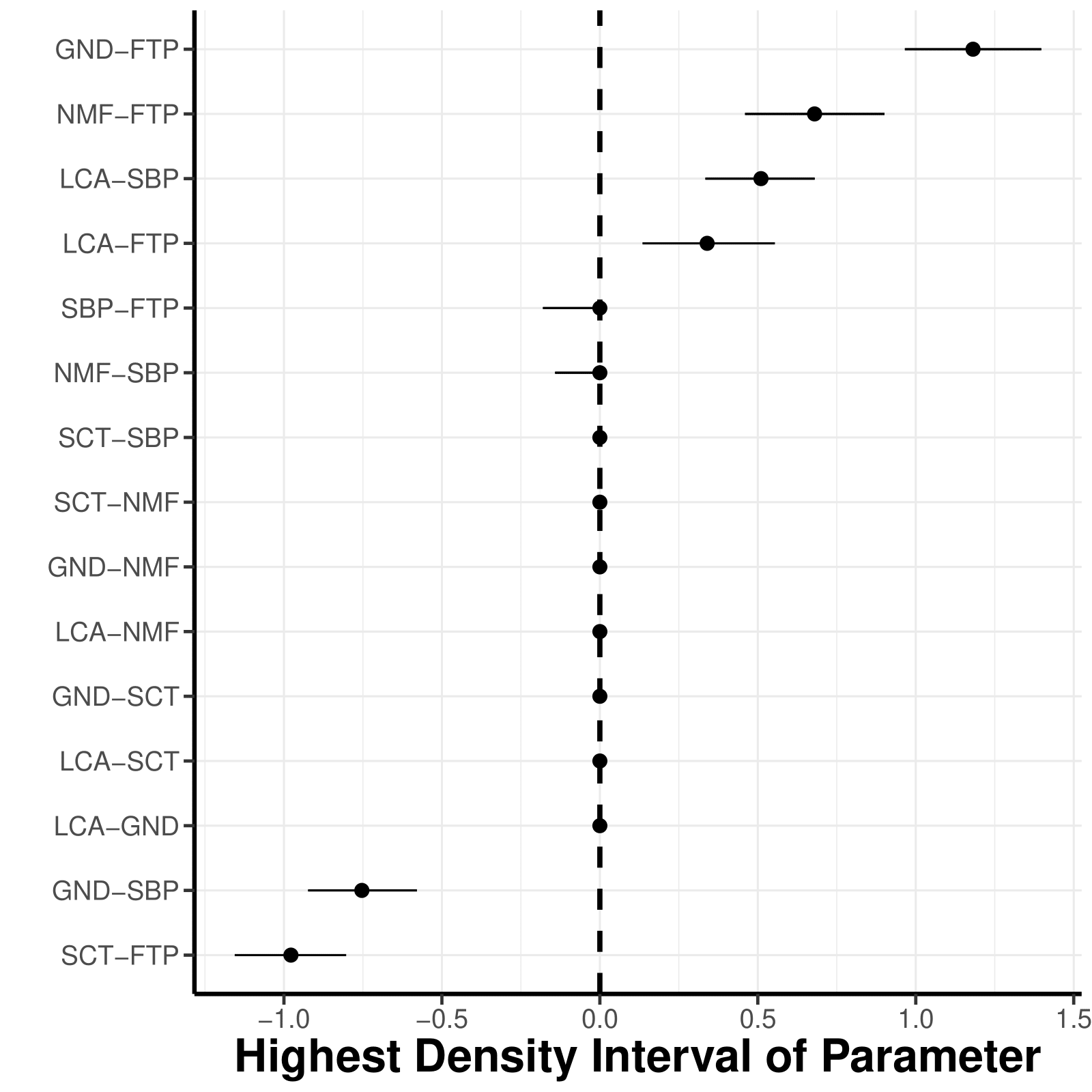
Furthermore, researcher can wish to aggregate the findings of the
network model, commonly done with centrality measures. Due to the
discussion around the meaningfulness of centrality measures in
psychometric network models, we recommend users to stick to the strength
centrality. To obtain the centrality measures, users need to set
save = TRUE and centrality = TRUE, when
estimating the network model with easybgm. The centrality
measures can be inspected with the centrality plot.
plot_centrality(res, measures = "Strength")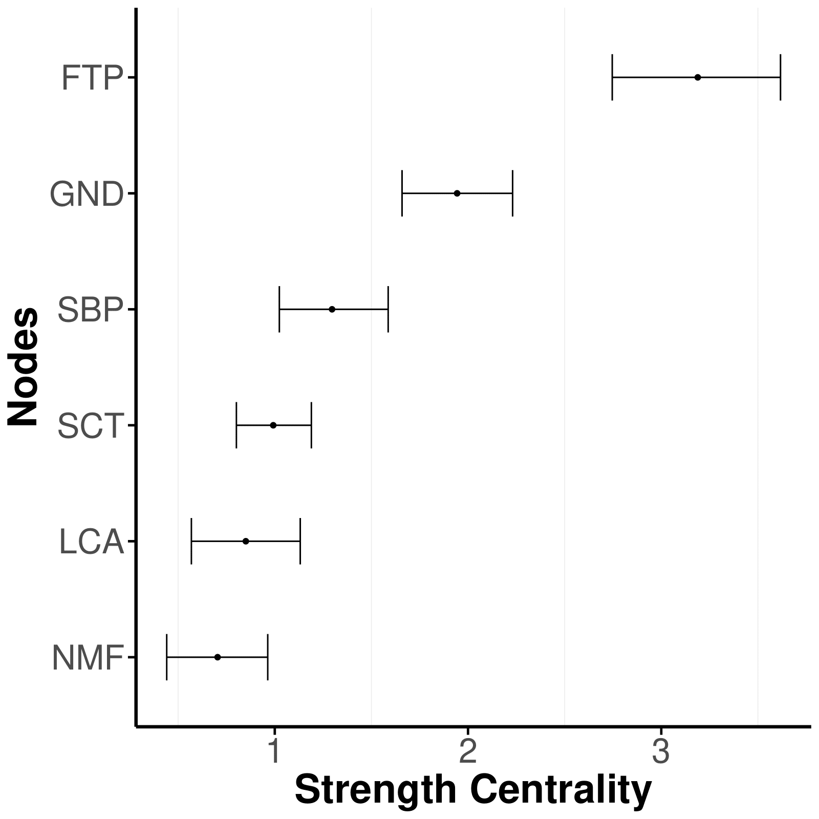
All of the functionalities mentioned above can also be used when
comparing networks across groups. The function
easybgm_compare allows users to compare networks across two
or more groups using Bayesian inference to extract differences in
conditional (in)dependence structures. The function supports the
packages BGGM and bgms.
library(easybgm)
library(bgms)

data <- na.omit(ADHD)

group1 <- data[1:10, 1:5]
group2 <- data[11:20, 1:5]

# for two groups
res <- easybgm_compare(list(group1, group2),
                type = "binary", save = TRUE)

# for multiple groups


res <- easybgm_compare(data[1:200, 1:5],
                group_indicator = rep(c(1, 2, 3, 4), each = 50),
                type = "binary",
                save = TRUE,
)For more information on the package, the Bayesian background, its application to networks and the respective plots, check out:
Huth, K., Keetelaar, S., Sekulovski, N., van den Bergh, D., & Marsman, M. (2023). Simplifying Bayesian analysis of graphical models for the social sciences with easybgm: A user-friendly R-package. https://doi.org/10.31234/osf.io/8f72p
Huth, K., de Ron, J., Luigjes, J., Goudriaan, A., Mohammadi, R., van Holst, R., Wagenmakers, E.J., & Marsman, M. (2023). Bayesian Analysis of Cross-sectional Networks: A Tutorial in R and JASP. PsyArXiv https://doi.org/10.31234/osf.io/ub5tc.
If you encounter any bugs or have ideas for new features, you can
submit them by creating an issue on Github. Additionally, if you want to
contribute to the development of easybgm, you can initiate
a branch with a pull request; we can review and discuss the proposed
changes.
Epskamp, S., Cramer, A. O. J., Waldorp, L. J., Schmittmann, V. D., & Borsboom, D. (2012). qgraph: Network Visualizations of Relationships in Psychometric Data. Journal of Statistical Software, 48 . doi: 10.18637/jss.v048.i04.
Huth, K., de Ron, J., Luigjes, J., Goudriaan, A., Mohammadi, R., van Holst, R., Wagenmakers, E.J., & Marsman, M. (2023). Bayesian Analysis of Cross-sectional Networks: A Tutorial in R and JASP. PsyArXiv doi: 10.31234/osf.io/ub5tc.
Marsman M, van den Bergh D, Haslbeck J.M.B. Bayesian Analysis of the Ordinal Markov Random Field. Psychometrika. 2025;90(1):146-182. doi: 10.1017/psy.2024.
Mohammadi, Reza, and Ernst C Wit. (2015). “BDgraph: An R Package for Bayesian Structure Learning in Graphical Models.” Journal of Statistical Software 89 (3). doi: 10.18637/jss.v089.i03.
Sekulovski, N., Arena, G., Haslbeck, J. M. B., Huth, K., Friel, N., & Marsman, M. (2025). A Stochastic Block Prior for Clustering in Graphical Models. PsyArXiv doi: 10.31234/osf.io/29p3m_v1.
Wickham, H. (2016). ggplot2: Elegant graphics for data analysis. Springer-Verlag New York. Retrixeved from https://ggplot2.tidyverse.org.
Williams, Donald R, and Joris Mulder. (2019). “Bayesian Hypothesis Testing for Gaussian Graphical Models: Conditional Independence and Order Constraints.” PsyArXiv. doi: 10.31234/osf.io/ypxd8.
Williams DR, Rast P, Pericchi LR, Mulder J (2020). Comparing Gaussian graphical models with the posterior predictive distribution and Bayesian model selection. Psychological Methods. doi: 10.1037/met0000254.
![]()