

![]()
The ofpetrial package allows the user to design
agronomic input experiments in a reproducible manner without using
ArcGIS or QGIS. The vignette for this
package provides more detailed guidance on how to use the package.
You can install the CRAN version of the ofpetrial
package.
install.packages("ofpetrial")You can install the development version of ofpetrial from Github:
devtools::install_github("DIFM-Brain/ofpetrial")Here, we demonstrate how to use the ofpetrial package to
create a single-input on-farm experiment trial design (more detailed
instructions on the basic workflow is provided in this
article).
library(ofpetrial)We start with specifying plot and machine information for inputs
using prep_plot.
n_plot_info <-
  prep_plot(
    input_name = "NH3",
    unit_system = "imperial",
    machine_width = 30,
    section_num = 1,
    harvester_width = 30,
    plot_width = 30
  )
#>
Now, we can create experiment plots based on them using
make_exp_plots().
exp_data <-
  make_exp_plots(
    input_plot_info = n_plot_info,
    boundary_data = system.file("extdata", "boundary-simple1.shp", package = "ofpetrial"),
    abline_data = system.file("extdata", "ab-line-simple1.shp", package = "ofpetrial"),
    abline_type = "free"
  )
#> Linking to GEOS 3.11.0, GDAL 3.5.3, PROJ 9.1.0;
#> sf_use_s2() is TRUE
#> Warning: There was 1 warning in `dplyr::mutate()`.
#> ℹ In argument: `experiment_plots_dissolved = list(...)`.
#> ℹ In row 1.
#> Caused by warning:
#> ! package 'sf' was built under R version 4.2.3

viz(exp_data, type = "layout", abline = TRUE)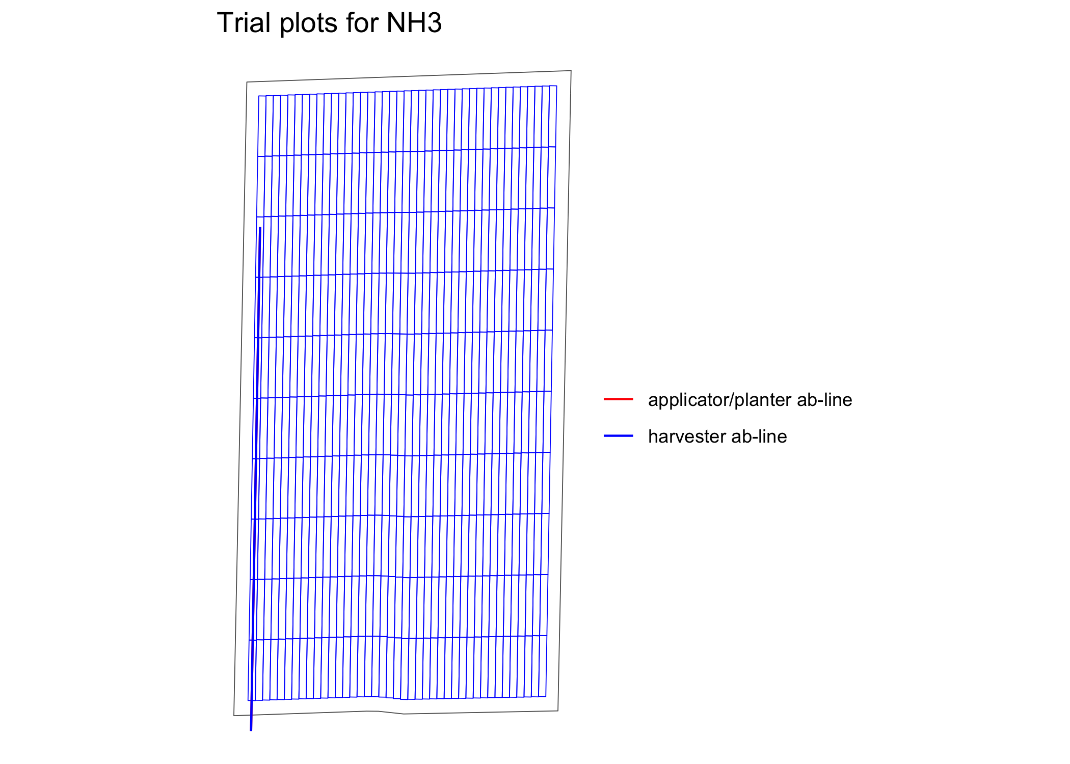
We first prepare nitrogen rates.
#!===========================================================
# ! Assign rates
# !===========================================================
n_rate_info <-
  prep_rate(
    plot_info = n_plot_info,
    gc_rate = 180,
    unit = "lb",
    rates = c(100, 140, 180, 220, 260),
    design_type = "ls",
    rank_seq_ws = c(5, 4, 3, 2, 1)
  )

dplyr::glimpse(n_rate_info)
#> Rows: 1
#> Columns: 12
#> $ input_name          <chr> "NH3"
#> $ design_type         <chr> "ls"
#> $ gc_rate             <dbl> 180
#> $ unit                <chr> "lb"
#> $ tgt_rate_original   <list> <100, 140, 180, 220, 260>
#> $ tgt_rate_equiv      <list> <82.0, 114.8, 147.6, 180.4, 2…
#> $ min_rate            <lgl> NA
#> $ max_rate            <lgl> NA
#> $ num_rates           <int> 5
#> $ rank_seq_ws         <list> <5, 4, 3, 2, 1>
#> $ rank_seq_as         <list> <NULL>
#> $ rate_jump_threshold <lgl> NA
We can now use assign_rates() to assign rates to
experiment plots.
trial_design <- assign_rates(exp_data, rate_info = n_rate_info)Here is the visualization of the trial design done by
viz.
viz(trial_design)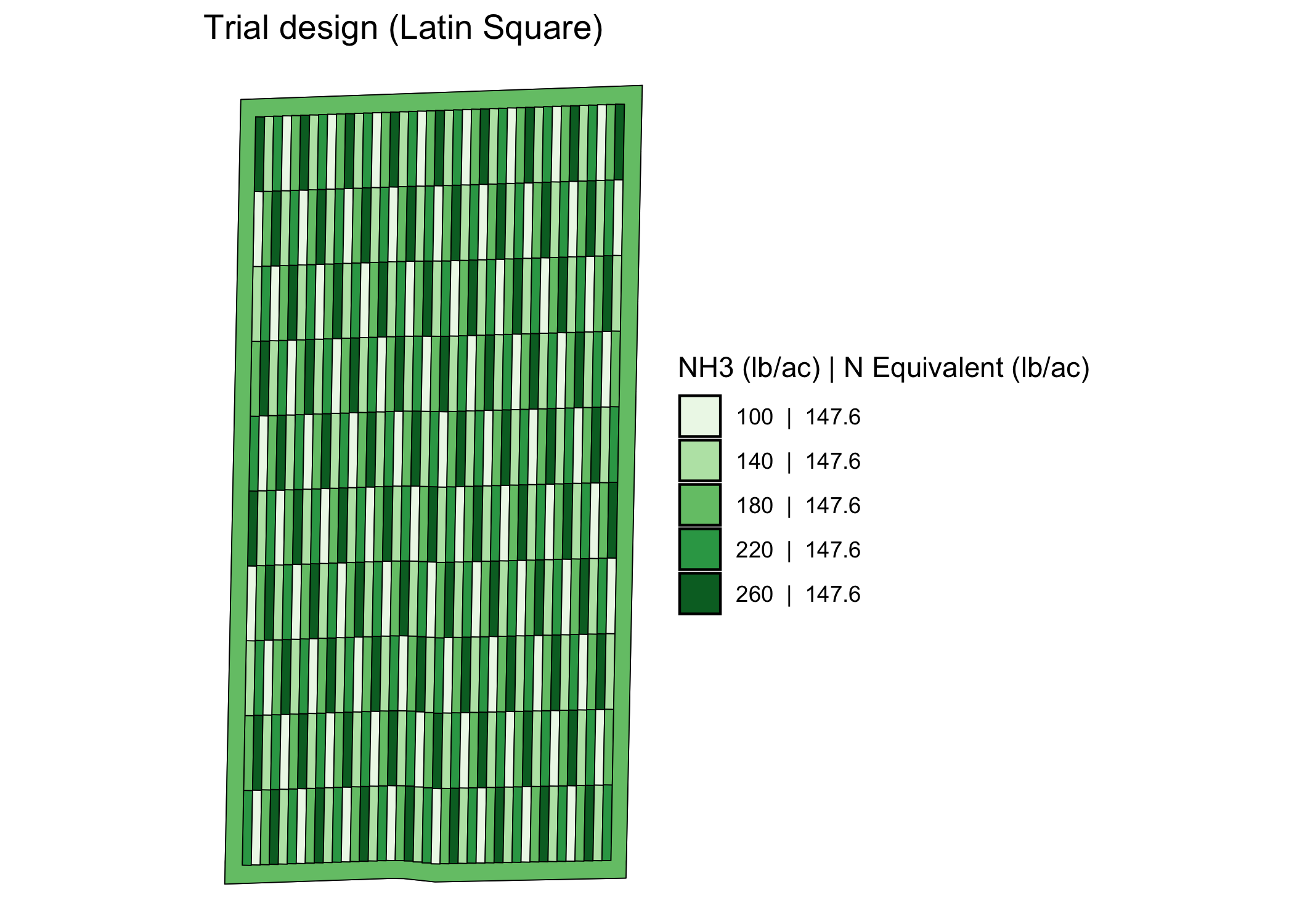
Along with the spatial pattern of the input rates, the applicator/planter ab-line and harvester ab-line are drawn by default.
You can write out the trial design as a shape file.
write_trial_files(td)This project was funded in part by a United States Department of Agriculture—National Institute of Food and Agriculture (USDA—NIFA) Food Security Program Grant (Award Number 2016-68004-24769) and by United States Department of Agriculture (USDA) -Natural Resources Conservation Service (NRCS), Commodity Credit Corporation (CCC), Conservation Innovation Grants On-Farm Conservation Innovation Trials (Award Number USDA-NRCS-NHQ-CIGOFT-20-GEN0010750).