
The ptetools package compartmentalizes the steps needed
to implement estimators of group-time average treatment effects (and
their aggregations) in order to make it easier to apply the same sorts
of arguments outside of their “birthplace” in the literature on
difference-in-differences.
Essentially, the idea is that many panel data causal inference problems involve steps such as:
Defining an identification strategy (e.g., difference-in-differences)
Defining a notion of a group (e.g., based on treatment timing)
Looping over groups and time periods
Organizing the data so that the correct data show up for each group and time period
Computing group-time average treatment effects (or other parameters that are local to a group and a time period)
Aggregating group-time average treatment effect parameters (e.g., into an event study or an overall average treatment effect parameter)
Many of these steps are common across different panel data causal inference settings. For example, you could implement a difference-in-differences identification strategy or a change-in-changes identification strategy with all of the same steps as above except for replacing step 1.
The idea of the ptetools package is to re-use as much
code/infrastructure as possible when developing new approaches to panel
data causal inference. For example, ptetools sits as the
“backend” for several other packages including: ife,
contdid, and parts of qte.
The main function is called pte. The most important
parameters that it takes in are subset_fun and
attgt_fun. These are functions that the user should pass to
pte.
subset_fun takes in the overall data, a group, a time
period, and possibly other arguments and returns a
data.frame containing the relevant subset of the data, an
outcome, and whether or not a unit should be considered to be in the
treated or comparison group for that group/time. There is one example of
a relevant subset function provided in the package: the
two_by_two_subset function. This function takes an
original dataset, subsets it into pre- and post-treatment periods and
denotes treated and untreated units. This particular subset is perhaps
the most common/important one for thinking about treatment effects with
panel data, and this function can be reused across applications.
The other main function is attgt_fun. This function
should be able to take in the correct subset of data, possibly along
with other arguments to the function, and report an ATT for
that subset. With minor modification, this function should be available
for most any sort of treatment effects application — for example, if you
can solve the baseline 2x2 case in difference in differences, you should
use that function here, and the ptetools package will take
care of dealing with the variation in treatment timing.
If attgt_fun returns an influence function, then the
ptetools package will also conduct inference using the
multiplier bootstrap (which is fast) and produce uniform confidence
bands (which adjust for multiple testing).
The default output of pte is an overall treatment effect
on the treated (i.e., across all groups that participate in the
treatment in any time period) and and event study. More aggregations are
possible, but these seem to be the leading cases; aggregations of
group-time average treatment effects are discussed at length in Callaway and
Sant’Anna (2021).
Below are several examples of how the ptetools package
can be used to implement an identification strategy with a very small
amount of new code.
The did
package, which is based on Callaway and
Sant’Anna (2021), includes estimates of group-time average treatment
effects, ATT(g,t), based on a difference in differences
identification strategy. The following example demonstrates that it is
easy to compute group-time average treatment effects using difference in
differences using the ptetools package. [Note:
This is definitely not the recommended way of doing this as there is
very little error handling, etc. here, but it is rather a proof of
concept. You should use the did package for this case.]
This example reproduces DID estimates of the effect of the minimum
wage on employment using data from the did package.
library(did)
data(mpdta)
did_res <- pte(
  yname = "lemp",
  gname = "first.treat",
  tname = "year",
  idname = "countyreal",
  data = mpdta,
  setup_pte_fun = setup_pte,
  subset_fun = two_by_two_subset,
  attgt_fun = did_attgt,
  xformla = ~lpop
)

summary(did_res)
#>
#> Overall ATT:
#>      ATT    Std. Error     [ 95%  Conf. Int.]
#>  -0.0305        0.0119    -0.0539     -0.0071 *
#>
#>
#> Dynamic Effects:
#>  Event Time Estimate Std. Error [95% Simult.  Conf. Band]
#>          -3   0.0298     0.0155       -0.0100      0.0695
#>          -2  -0.0024     0.0136       -0.0372      0.0323
#>          -1  -0.0243     0.0172       -0.0683      0.0198
#>           0  -0.0189     0.0127       -0.0514      0.0136
#>           1  -0.0536     0.0156       -0.0936     -0.0136 *
#>           2  -0.1363     0.0347       -0.2252     -0.0473 *
#>           3  -0.1008     0.0387       -0.1999     -0.0017 *
#> ---
#> Signif. codes: `*' confidence band does not cover 0
ggplot2::autoplot(did_res)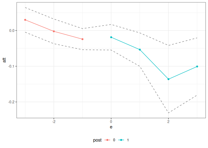
What’s most interesting here, is that the only “new” code that needs
to be written is in the
did_attgt function. You will see that this is a very
small amount of code.
As a next example, consider trying to estimate effects of COVID-19 related policies during a pandemic. The estimates below are for the effects of state-level shelter-in-place orders during the early part of the pandemic.
The data for this example is included in the ptetools
package:
data(covid_data)Callaway and Li (2021) argue that a particular unconfoundedness-type strategy is more appropriate in this context than DID-type strategies due to the spread of COVID-19 cases being highly nonlinear. However, they still deal with the challenge of variation in treatment timing. Therefore, it is still useful to think about group-time average treatment effects, but the DID strategy should be replaced with their particular unconfoundedness type assumption.
The ptetools package handles this through
pte_default with
lagged_outcome_cov = TRUE.
# formula for covariates
xformla <- ~ current + I(current^2) + region + totalTestResults
covid_res <- pte_default(
yname = "positive",
gname = "group",
tname = "time.period",
idname = "state_id",
data = covid_data2,
xformula = xformla,
d_outcome = FALSE,
lagged_outcome_cov = TRUE,
max_e = 21,
min_e = -10
)
summary(covid_res)
#>
#> Overall ATT:
#> ATT Std. Error [ 95% Conf. Int.]
#> -13.2547 88.0238 -185.7783 159.2689
#>
#>
#> Dynamic Effects:
#> Event Time Estimate Std. Error [95% Simult. Conf. Band]
#> -10 -6.3170 6.2253 -21.9441 9.3101
#> -9 2.1087 1.0403 -0.5026 4.7200
#> -8 -2.7721 1.3161 -6.0759 0.5316
#> -7 3.8965 2.2331 -1.7091 9.5021
#> -6 -1.0588 2.6737 -7.7703 5.6527
#> -5 2.4337 5.8718 -12.3058 17.1732
#> -4 0.2436 1.6735 -3.9574 4.4446
#> -3 -1.3052 4.2679 -12.0187 9.4083
#> -2 0.4594 2.1419 -4.9173 5.8362
#> -1 4.0376 2.6016 -2.4931 10.5682
#> 0 -3.2518 3.0698 -10.9577 4.4542
#> 1 -7.4231 9.9500 -32.3999 17.5537
#> 2 -0.3148 8.5038 -21.6614 21.0318
#> 3 2.7880 8.3010 -18.0496 23.6256
#> 4 1.3625 11.3570 -27.1462 29.8713
#> 5 -2.9563 19.9698 -53.0854 47.1727
#> 6 -17.2610 28.2230 -88.1075 53.5855
#> 7 -19.2258 36.3255 -110.4116 71.9599
#> 8 -21.5150 40.3927 -122.9103 79.8804
#> 9 -25.2793 37.7454 -120.0294 69.4707
#> 10 -23.0541 49.5949 -147.5491 101.4409
#> 11 -3.8346 47.0793 -122.0149 114.3456
#> 12 -5.6789 61.7977 -160.8060 149.4482
#> 13 -12.4977 93.6276 -247.5254 222.5299
#> 14 -19.6199 91.2854 -248.7680 209.5283
#> 15 -11.6638 87.2393 -230.6552 207.3275
#> 16 -15.0522 101.3735 -269.5237 239.4193
#> 17 -3.3234 122.7752 -311.5184 304.8716
#> 18 -14.3328 110.3989 -291.4603 262.7947
#> 19 -26.1852 145.9644 -392.5905 340.2201
#> 20 -40.7039 139.8987 -391.8830 310.4753
#> 21 -58.7364 154.9435 -447.6815 330.2087
#> ---
#> Signif. codes: `*' confidence band does not cover 0
ggplot2::autoplot(covid_res) + ylim(c(-1000, 1000))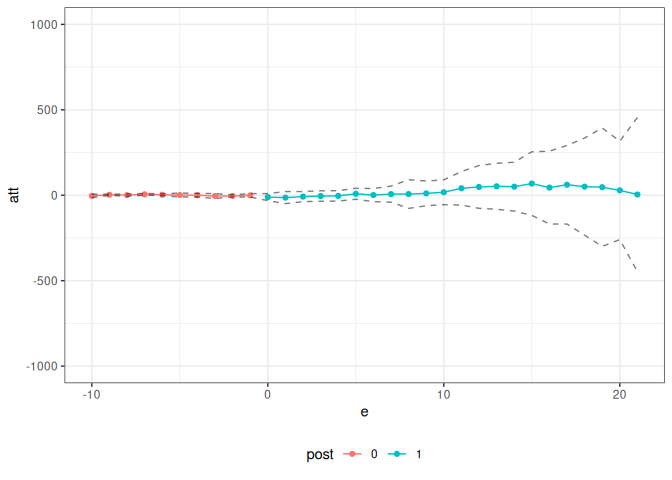
What’s most interesting is just how little code needs to be written
here. The pte_default function handles the
unconfoundedness-type identification strategy directly, with no custom
attgt_fun required.
The code above used the multiplier bootstrap. The great thing about the multiplier bootstrap is that it’s fast. But in order to use it, you have to work out the influence function for the estimator of ATT(g,t). Although I pretty much always end up doing this, it can be tedious, and it can be nice to get a working version of the code for a project going before working out the details on the influence function.
The ptetools package can be used with the empirical
bootstrap. There are a few limitations. First, it’s going to be
substantially slower. Second, this code just reports pointwise
confidence intervals. However, this basically is set up to fit into my
typical workflow, and I see this as a way to get preliminary
results.
Let’s demonstrate it. To do this, consider the same setup as in Example 1, but where no influence function is returned. Let’s write the code for this:
# did with no influence function
did_attgt_noif <- function(gt_data, xformla, ...) {
  # call original function
  did_gt <- did_attgt(gt_data, xformla, ...)

  # remove influence function
  did_gt$inf_func <- NULL

  did_gt
}
Now, we can show the same sorts of results as above
did_res_noif <- pte(
  yname = "lemp",
  gname = "first.treat",
  tname = "year",
  idname = "countyreal",
  data = mpdta,
  setup_pte_fun = setup_pte,
  subset_fun = two_by_two_subset,
  attgt_fun = did_attgt_noif, # this is only diff.
  xformla = ~lpop
)

summary(did_res_noif)
#>
#> Overall ATT:
#>      ATT    Std. Error     [ 95%  Conf. Int.]
#>  -0.0323        0.0129    -0.0582     -0.0063 *
#>
#>
#> Dynamic Effects:
#>  Event Time Estimate Std. Error [95% Simult.  Conf. Band]
#>          -3   0.0269     0.0139       -0.0003      0.0541
#>          -2  -0.0050     0.0123       -0.0290      0.0191
#>          -1  -0.0229     0.0144       -0.0511      0.0054
#>           0  -0.0201     0.0123       -0.0443      0.0040
#>           1  -0.0547     0.0176       -0.0892     -0.0203 *
#>           2  -0.1382     0.0403       -0.2172     -0.0592 *
#>           3  -0.1069     0.0357       -0.1769     -0.0369 *
#> ---
#> Signif. codes: `*' confidence band does not cover 0
ggplot2::autoplot(did_res_noif)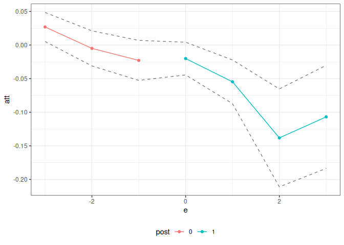
What’s exciting about this is just how little new code needs to be written.