



Shift-share / Bartik IV analysis in R is currently spread across
several single-purpose tools, each of which has its own data
conventions. ssBartik connects those steps into one
consistent workflow: (a) construct variables → (b) diagnose → (c)
estimate → (d) infer → (e) visualize, organized around the two
identification routes of the modern literature (i.e., exogenous
shift and exogenous share
approaches).
Once you pick the identification route with a single argument
(exogenous = "share" or "shift"), everything
downstream follows through simple functions.
ssBartik turns estimation and diagnostic results into
publication-ready figures and tables. The examples below demonstrate
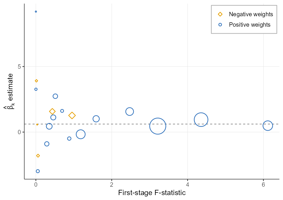
some of the package’s main outputs using sample datasets. The first
model figure follows visualization in Goldsmith-Pinkham, Sorkin, and
Swift (2020).

# install.packages("remotes")
remotes::install_github("takuma1102/ssBartik")
You can also install through R-universe.
install.packages(
  "ssBartik",
  repos = c("https://takuma1102.r-universe.dev", getOption("repos"))
)
ShiftShareSE by Prof. Michal Kolesár (for AKM/AKM0
inference) is optional and used when installed.
The ssBartik function builds the dataset for shift-share
IV analysis, runs the full pipeline, and produces results regarding a CI
comparison between AKM/AKM0 and conventional methods, a calculation of
the effective F, an overidentification test, Rotemberg weights, a
pre-trend test, a placebo analysis, and an LOO analysis.
library(ssBartik)
pipeline_analysis <- ssbartik(data = data, shares = shares, shocks = shocks, controls = "w1", weights = "pop",
                exogenous = "share",     # or "shift"
                covariates = "w1",
                pre_y = "ypre", placebo_y = "yplac")
print(pipeline_analysis)                   # printed estimate + diagnostics
The instrument z_i = Σ_n s_{in} g_n is
constructed identically whichever route you take. The
exogenous flag governs which diagnostics and controls
apply:
| step | exogenous = "share" (GPSS) |
exogenous = "shift" (AKM, BHJ) |
|---|---|---|
| headline diagnostic | Rotemberg weights + figure | effective shocks / exposure concentration |
| credibility check | share balance vs. observables | shock balance vs. characteristics |
| cross-instrument | overidentification across β_k | location ↔︎ shock IV equivalence |
| pre-period / placebo | pre-trend + placebo outcome | pre-trend + placebo outcome |
| robustness | leave-one-out, drop-top-n, randomization inference | leave-one-out, drop-top-n, randomization inference |
| extra control | — | sum-of-shares (auto, when incomplete) |
| inference | EHW / cluster / AKM / AKM0 (iid, two-way on request) | EHW / cluster / AKM / AKM0 (iid, two-way on request) |
With a design in hand, each credibility check is finished through a single call.
d   <- ssb_design(df$data, df$shares, df$shocks,
                  controls = "w1", weights = "pop", exogenous = "share")
rot <- ssb_rotemberg(d)                    # Rotemberg-weight decomposition
plot(rot, n = 6)                           # see below
est <- ssb_estimate(d)                     # EHW / cluster / AKM / AKM0 (add iid/two-way on request)
ssb_plot_ci(est)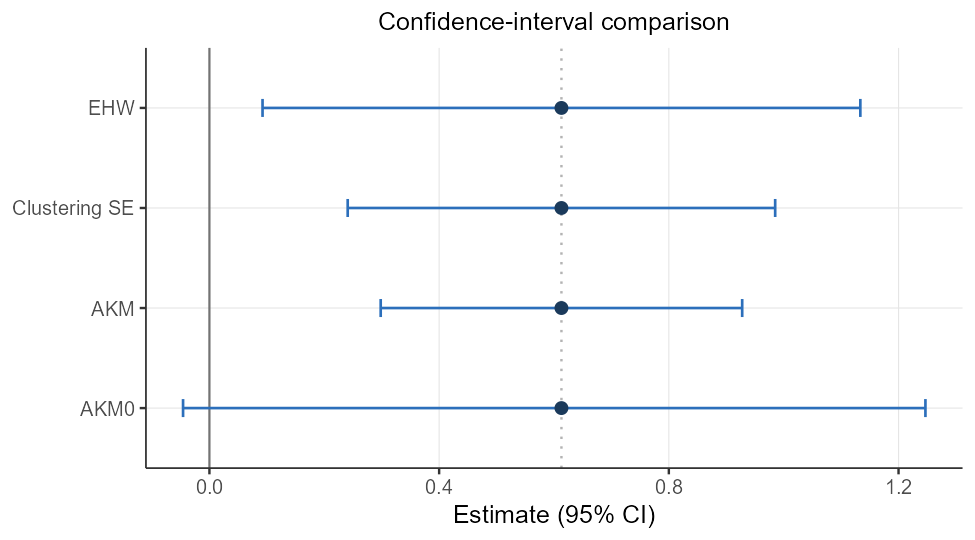
# instrument strength & internal consistency
ssb_first_stage(d)               # standard robust F + exposure-robust "effective" F
ssb_equivalence(d)               # location-level SSIV == shock-level IV (sanity check)
ssb_overid(d)                    # do the per-share estimates agree? (Cochran's Q)
# identifying-assumption checks
ssb_shock_balance(d, shock_covariates = sc)  # shocks vs. pre-determined characteristics
ssb_pretrend(d, pre_y = "y_pre")             # does exposure predict pre-trends?
ssb_placebo(d, placebo_y = "y_plac")         # full IV on an outcome that shouldn't move
ssb_ri(d, R = 999, block = "grp") # AR-style randomization inference (shocks permuted within blocks)
# sensitivity to influential shocks
ws<- ssb_weight_summary(d, covariates = "w1")     # who carries the weight? (α vs. βₖ, F, covariates)
plot(ws)
ssb_drop_top(d, n = 5)                        # re-estimate without the top-weight shocks
ssb_recenter(d, method = "permute", block = "grp")     # block-wise recentering (within-block mean shock)
Each returns a small object with a readable print()
method; the same checks run automatically inside ssbartik()
/ ssb_pipeline() when you pass the corresponding arguments
(pre_y, placebo_y,
shock_covariates, covariates).
Construct
| function | purpose |
|---|---|
ssb_design() |
define a shift-share design (entry point) |
ssbartik() / ssb_pipeline() |
one-call pipeline (from raw data / from an existing design) |
Diagnose
| function | purpose |
|---|---|
ssb_rotemberg() |
Rotemberg-weight decomposition (+
format()/plot() paper table) (see GPSS) |
ssb_weight_summary() |
Rotemberg-weight summary + correlations (α vs. βₖ, F, covariates) |
ssb_shock_summary() |
effective number of shocks, exposure concentration |
ssb_first_stage() |
first-stage strength: standard & exposure-robust (effective) F |
Note The Rotemberg decomposition is the headline credibility table of the exogenous-shares approach (Goldsmith-Pinkham, Sorkin & Swift 2020): it shows which shocks the estimate leans on and whether their just-identified estimates agree.
ssb_rotemberg()prints a console summary by default, and exports a publication-quality table of the top-weight shocks on demand:
rot <- ssb_rotemberg(d)
print(rot)                                 # console summary (default)

writeLines(format(rot, "latex"))           # paste-ready booktabs LaTeX
writeLines(format(rot, "markdown"))        # GitHub pipe table
print(rot, format = "latex", n = 8)        # same, straight from print()

plot(rot, file = "rotemberg_table.png")    # compact booktabs image (.png/.pdf); see below
Estimate & infer
| function | purpose |
|---|---|
ssb_estimate() |
point estimate + CI: EHW/cluster/AKM/AKM0 by default, iid/two-way on
request (+ format() paper table) (see AKM) |

| function | purpose |
|---|---|
ssb_aggregate() / ssb_shock_iv() |
shock-level aggregation and shock-level IV |
ssb_equivalence() |
location-level ↔︎ shock-level IV equivalence check |
Credibility & robustness checks
| function | purpose |
|---|---|
ssb_overid() |
overidentification / cross-instrument homogeneity test |
ssb_share_balance() |
share-vs-observables balance (share route) |
ssb_shock_balance() |
shock-vs-characteristics balance (shift route) |
ssb_pretrend() |
pre-trend test (reduced form of a pre-period outcome on the instrument) |
ssb_placebo() |
placebo-outcome test (full IV on an outcome that should not move) |
ssb_ri() |
randomization inference (Anderson-Rubin-style placebo shocks) |
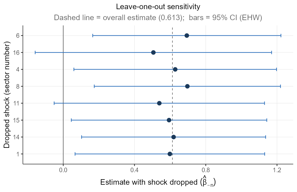
ssb_loo() |
leave-one-sector-out sensitivity (see AKM) |
| function | purpose |
|---|---|
ssb_drop_top() |
re-estimate after dropping the top-weight shocks together |
ssb_recenter() |
recentering — demean or block-wise permute (Borusyak & Hull) |
Visualize
| function | purpose |
|---|---|
ssb_plot_rotemberg() / ssb_plot_ci() |
Rotemberg bubble chart / confidence-interval comparison |
ssb_plot_loo() / ssb_plot_ri() |
leave-one-out sensitivity / randomization-inference null |
ssb_plot_overid() / ssb_plot_shocks() |
just-identified estimate dispersion / exposure Lorenz curve |

| function | purpose |
|---|---|
autoplot() |
method for any of the figures above |
Note 1:
ssb_plot_rotemberg()reproduces the canonical Goldsmith-Pinkham–Sorkin–Swift diagnostic: each sector’s just-identified estimate against its first-stage F-statistic, bubble area proportional to the absolute Rotemberg weight, positive weights as blue open circles and negative as amber open diamonds, with the overall estimate marked by the dashed line.
Note 2:
ssb_plot_ci()puts the point estimate next to every method’s interval, with the axis always including the null at 0, so both the practical cost of the exposure-robust correction and each method’s verdict on significance are immediate. The comparison is of intervals: AKM0 is defined directly as a (possibly asymmetric) interval, so it is the interval — not a standard error — that matters. (In this example the naive/EHW interval excludes 0 while AKM0 does not.)
Experimental, but the output schema is intended to be stable. Pin package versions in production code.
When developing ssBartik, I gratefully referenced tools
built by others: ShiftShareSE
(Michal Kolesár), ssaggregate
(Kyle Butts), bartik.weight
(JJ Chern), and bartik-weight
(Paul Goldsmith-Pinkham for Stata and R). Kudos to their authors for
making these ideas legible and reproducible.
To keep the package lightweight and close to base R,
ssBartik depends on only ShiftShareSE, listed
under Suggests and called solely for the AKM / AKM0 exposure-robust
standard errors. The other three packages above are neither imported nor
called. They served purely as references and the functionality they
built is reimplemented natively in ssBartik in base R so
that external dependencies stay minimal.
Please also cite whichever underlying methods and tests you actually used.
MIT © 2026 Takuma Iwasaki (Stanford University).