tabular

tabular turns a pre-summarised data frame into a submission-grade clinical table and emits it natively to RTF, PDF, HTML, LaTeX, Typst, and DOCX — no Java, no LibreOffice, no Word automation. One short pipeline gives you decimal alignment via real font metrics, multi-level column headers, predicate-targeted styling, and group-aware pagination, built for CDISC ADaM workflows and FDA / EMA / PMDA submissions.

It is the only R table package that pairs a live HTML preview with a paginated print deliverable: the same spec you eyeball in a notebook is the one that paginates into the RTF you ship.

Scope. tabular renders the full set of clinical outputs – tables, listings, and figures (the “T”, “L”, and “F” of TFL) – to RTF, LaTeX, Typst, HTML, PDF, and DOCX from one verb pipeline. A zero-row table renders an empty-data placeholder (“No data available to report”) in the body, with the page chrome and column headers intact.

Installation

Install the released version from CRAN:

install.packages("tabular")

Or the development version from GitHub:

# install.packages("pak")
pak::pak("vthanik/tabular")
# or
remotes::install_github("vthanik/tabular")

R dependencies install automatically. The backends differ in what else they need:

PDF is the only backend that shells out, and it has two engines:

• LaTeX — emit(spec, "out.pdf") compiles via xelatex when a usable TeX is found. tabularray + ninecolors ship with tabular, so no tlmgr_install() step is needed even on locked-down servers (Domino, Posit Workbench) where tlmgr install is impossible.
• Typst — with no usable TeX, emit() falls back to the typst compiler (the standalone binary, or the copy bundled inside Quarto, which ships with RStudio / Posit Workbench). No TeX installation at all, and compiles in well under a second.

Pass format = "latex" or format = "typst" to pick an engine explicitly; with neither engine present, install one:

install.packages("tinytex")
tinytex::install_tinytex(bundle = "TinyTeX") # one-time TeX setup
# or: install Quarto (https://quarto.org) — it bundles the typst engine

check_latex() reports which LaTeX packages resolve (probed through kpsewhich, the same resolver xelatex uses) and prints the remedy for anything genuinely missing; check_typst() does the same for the typst engine (binary, version floor, and the font chain PDFs render in); check_fonts(spec) audits the fonts a spec asks for, per backend.

tabular::check_latex()   # LaTeX-PDF readiness, with the install remedy
tabular::check_typst()   # Typst-PDF readiness (no TeX needed)

TeX Live on a managed OS. If TeX Live came from the system package manager (RHEL dnf, Debian/Ubuntu apt), its tlmgr is usually locked and tlmgr_install() fails on permissions. Install user-space TinyTeX alongside it rather than fighting the system copy — and never reach for --ignore-warning to force it.

A table in one pipeline

The pipeline starts from a pre-summarised wide data frame (one row in = one display row — tabular does no aggregation) and chains one verb per concern. Every verb returns an updated, immutable tabular_spec; the engine resolves it at render time.

library(tabular)

# BigN denominators, keyed by arm
n <- stats::setNames(cdisc_saf_n$n, cdisc_saf_n$arm_short)

# columns render in data-frame order, so put them in dose order first;
# subset to Age / Sex / Race for a compact display
keep <- c("Age (years)", "Sex, n (%)", "Race, n (%)")
demo <- cdisc_saf_demo[
  cdisc_saf_demo$variable %in% keep,
  c("variable", "stat_label", "placebo", "drug_50", "drug_100", "Total")
]

tab <- tabular(
  demo,
  titles = c(
    "Table 14.1.1",
    "Demographic and Baseline Characteristics",
    "Safety Population"
  ),
  footnotes = "Percentages are based on the number of subjects per treatment group."
) |>
  cols(
    variable = "Characteristic",
    stat_label = "Statistic",
    placebo = col_spec(
      label = "Placebo (N={n['placebo']})",
      align = "decimal"
    ),
    drug_50 = col_spec(
      label = "Drug 50 (N={n['drug_50']})",
      align = "decimal"
    ),
    drug_100 = col_spec(
      label = "Drug 100 (N={n['drug_100']})",
      align = "decimal"
    ),
    Total = col_spec(label = "Total (N={n['Total']})", align = "decimal")
  ) |>
  group_rows(by = "variable")

# render to any backend by file extension (or format = "...")
path <- emit(tab, tempfile(fileext = ".rtf")) # submission deliverable

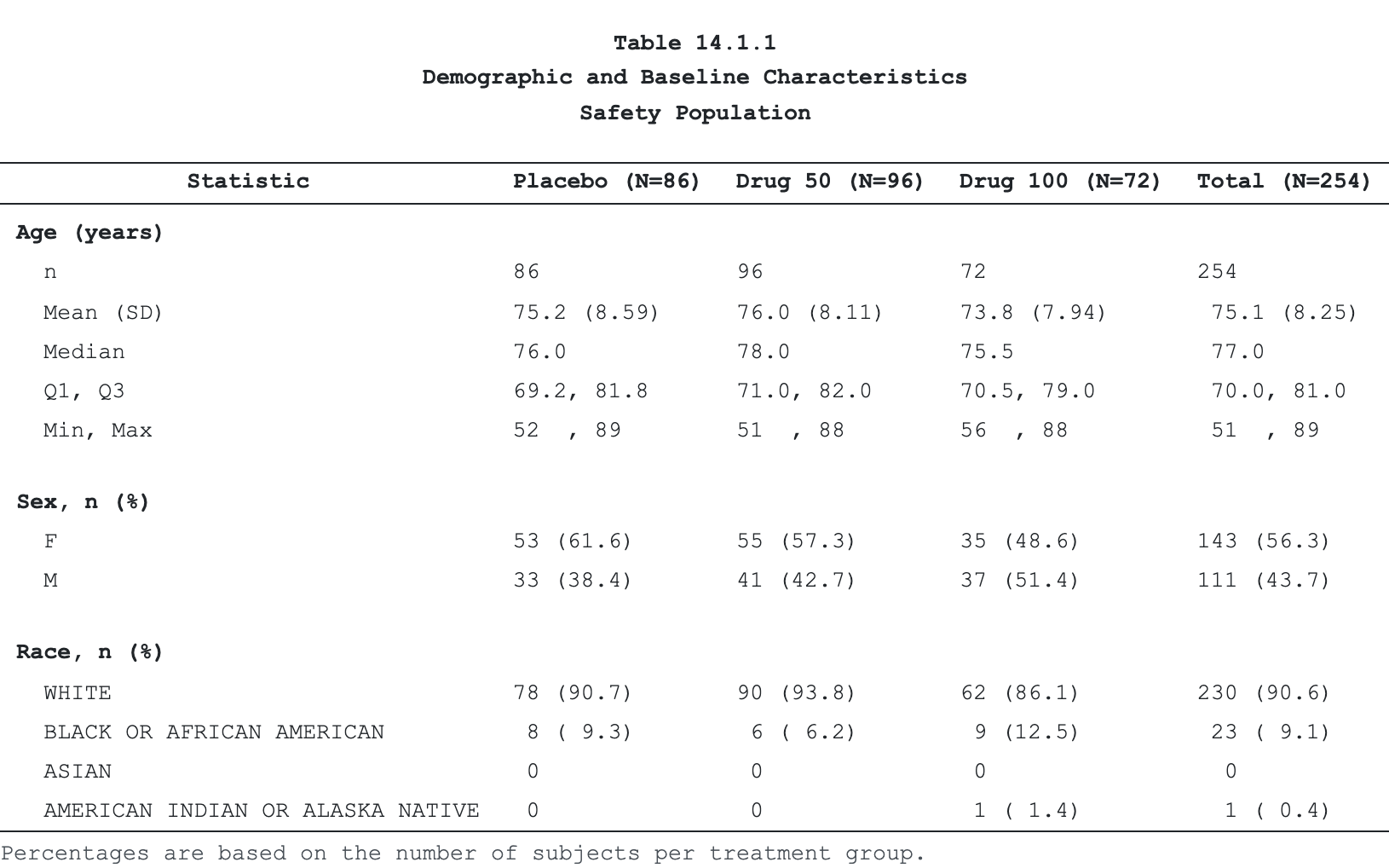
The same tab emits to every backend from the one spec. The table below is tabular’s own HTML render — the identical spec also produces RTF, a paginated PDF (LaTeX- or typst-compiled), a tabularray LaTeX fragment, a native Typst document, and native OOXML .docx:

Why tabular?

• Every native backend, one spec. emit() dispatches on the file extension to RTF 1.9.1, self-contained Bootstrap HTML, tabularray LaTeX, native Typst, native OOXML DOCX, and PDF — compiled through LaTeX when a TeX is installed, or through the typst engine (bundled with Quarto) on TeX-less machines. No JVM, no Office round-trip.
• Decimal alignment that survives the page. Numbers align on the decimal using the backend’s real font metrics, not guessed padding — so columns stay aligned in print, not just on screen.
• Submission chrome built in. Multi-line titles, up to eleven footnote lines, page header/footer slots, and the four-section page layout regulatory reviewers expect.
• Auto-numbered footnotes. footnote() anchors a marker to any cell, header, or title; the engine assigns the glyph once, in reading order, deduped by id, and byte-identical across every backend and page.
• Group-aware pagination. Keep a SOC and its preferred terms on one page, repeat titles/headers/footnotes per page, control orphan/widow rows, and split wide tables into horizontal panels.
• Display-only by design. tabular styles and renders; it never filters, aggregates, or weights. Pair it with cards / gtsummary / dplyr / SAS upstream and feed it a tidy wide frame.
• A QC trail. emit(data_file = ...) writes the resolved wide data beside the render, and a CDISC ARS audit manifest documents the display.

Where tabular fits

tabular is a renderer for pre-summarised clinical tables, not a statistics engine. Compute the summary upstream — with cards, gtsummary, dplyr, or SAS — then hand the finished wide frame to tabular(). Reach for gtsummary or rtables when you want the package to compute the summary; reach for tabular to render a summary you already have to submission-grade output.

The matrix reflects each package’s documented export surface (verified against their namespaces; via gt means gtsummary renders through gt):

Two notes on the marks:

• Live HTML preview means the table renders as HTML inline when you print it in a Quarto / R Markdown chunk or the RStudio viewer (a knit_print method). rtables prints a monospace ASCII table by default and ships no knit_print method, so it is — here; it can still emit HTML through an explicit as_html() call.
• PDF is compiled through LaTeX, so it needs a TeX installation — see Installation above. Every other backend is pure R.

Documentation

• Get started — the mental model and your first table
• Data in — turn a cards/cardx ARD into the wide frame with pivot_across()
• Structure — columns, headers, BigN, and pagination
• Presentation — titles, footnotes, page chrome, and styling
• Output & qualification — backends, requirements, and the CDISC-pilot validation
• Reference — every verb, grouped by role

License

MIT © Vignesh Thanikachalam