


🇧🇷 Novidade: acompanhe os resultados atualizados do agregador
Bayesian State-Space Aggregation of Brazilian Presidential Polls
As presidential elections approach, Brazilian voters are confronted
with a growing volume of conflicting polling estimates, each employing
distinct methodologies and sampling designs. agregR
provides a rigorous framework to filter the surfeit of data and uncover
the underlying level of support for each candidate.
The package implements a set of Bayesian state-space models in Stan to normalize polling data from sources that are noisy and possibly biased. It features methods to account for:
agregR is built on CmdStan, the
state-of-the-art backend for Stan. Since CmdStan is not available on
CRAN (and
will likely never be), it needs to be installed separately. This
one-time setup yields substantial gains in compilation speed and
sampling performance.
We recommend following these installation steps in order:
Windows users must first install RTools to
enable C++ compilation. MacOS requires Xcode
Command Line Tools, and Linux users should install
the distribution-specific compiler (e.g., Ubuntu:
sudo apt install build-essential).
The most convenient way to install CmdStan is via the
cmdstanr interface.
# Install cmdstanr interface
install.packages("cmdstanr", repos = c("https://stan-dev.r-universe.dev", "https://cloud.r-project.org"))

# Install CmdStan
cmdstanr::install_cmdstan()
Optional: make sure everything is in place.
cmdstanr::check_cmdstan_toolchain()agregRYou can install the stable version of agregR from CRAN
with:
install.packages("agregR", type = "source")Experimental: the development (and possibly
unstable) version of agregR can be installed with:
if (!require(pak)) install.packages("pak")
pak::pak("rnmag/agregR")The main function rodar_agregador() centralizes data
preparation, model compilation, and sampling. It returns the full
CmdStanMCMC objects for diagnostics, along with tidy data
frames for house effects and daily voting estimates.
library(agregR)

# Execute the aggregation pipeline for a 2nd round scenario
result <- rodar_agregador(
  data_inicio = "01/06/2025",
  turno = 2,
  cenario = "Lula vs Flávio",
  modelo = "Viés Relativo com Pesos"
)

# Daily voting estimates + poll data in tidy format
result$votos_estimados

# House effects in tidy format
result$vies_institutos

# Raw model object
result$modelo_brutoThe package includes a suite of plots designed for public communication.
We strongly recommend RStudio users to enable
the AGG graphics device in
Options -> General -> Graphics -> Backend.
Visualizes the estimated voting intention for each candidate overlaying the raw polling data.
grafico_agregador(result)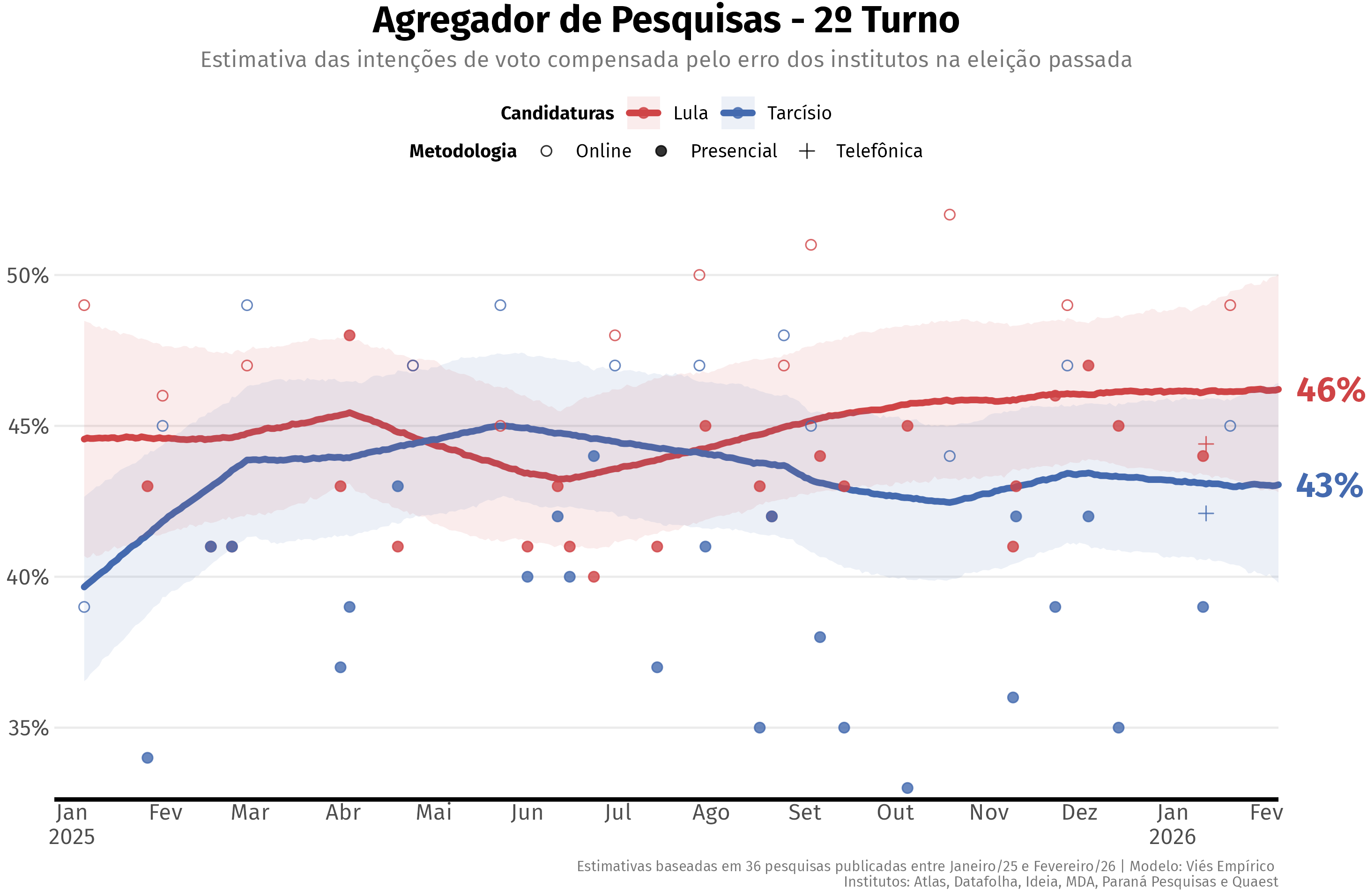
Visualizes the systematic bias for each institute, identifying consistent directional skews.
grafico_vies(result, candidaturas = c("Lula", "Flávio"))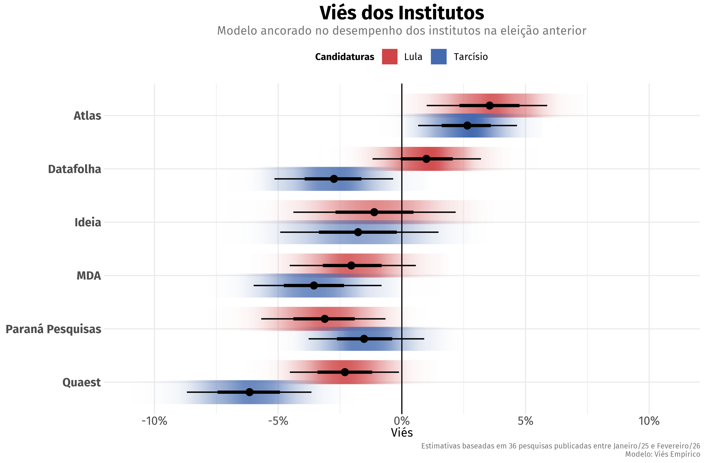
Visualizes how the data has informed the model by comparing prior vs. posterior distributions for selected parameters.
grafico_priori_posteriori(result, tipo = "Viés", candidaturas = c("Lula", "Flávio"))
The package offers configuration functions for fine-grained control
over plots and models. Configuration values can be stored in new objects
using the functions configurar_agregador(),
configurar_prioris() and configurar_grafico().
Alternatively, they can be passed directly as lists to the appropriate
arguments.
# Config passed as list: longer run with tighter priors for non-sampling error
result_custom <- rodar_agregador(
  turno = 2,
  cenario = "Lula vs Flávio",
  config_agregador = list(stan_chains = 4,
                          stan_iter = 2000,
                          stan_warmup = 2000),
  config_prioris = list(sd_tau_priori = 0.01)
)

# Config passed as function: custom color and custom symbols
grafico_agregador(
  result,
  config_grafico = configurar_grafico(
    cores_candidaturas = c("Flávio" = "yellow"),
    simbolos = c("Presencial" = 19, "Online" = 2, "Telefônica" = 4)
  )
)

# Config passed as object: custom color
config_custom <- configurar_grafico(cores_candidaturas = c(Lula = "green"))

grafico_agregador(result, config_grafico = config_custom)We are interested in performing inference on the latent state of public opinion: the dynamic, unobserved level of support for each candidate. Polls are periodic snapshots of this state, but the pictures are distorted and grainy.
An apt analogy is a GPS receiver navigating an area with spotty connectivity. It receives sparse, conflicting pings from different satellites, each with its own uncertainty due to corrupted data packages, equipment miscalibration or inherent manufacturer bias. The system must achieve three objectives:
Much like satellites, pollsters might be miscalibrated. Their
readings contain noise introduced by different sampling designs,
weighting protocols, and question wording, among other factors.
agregR shares the same objectives as the GPS receiver:
The methods implemented by agregR build on Jackman
(2009). They are variously known as state-space models (SSM), dynamic
linear models (DLM) or Kalman filters and consist of two integrated
components:
The latent voting intention for each candidate updates daily according to a local linear trend. The evolution of the latent state through time \(t\) for candidate \(c\) is governed by the level component \(\mu_{t, c}\) and influenced by the trend component \(\nu_{t, c}\).
The level \(\mu_{t, c}\) is defined by the previous state \(\mu_{t - 1, c}\) plus the trend \(\nu_{t - 1, c}\), subject to stochastic level innovations \(\eta_{t, c}\). The trend itself evolves as a random walk driven by innovations \(\zeta_{t, c}\).
\[ \begin{pmatrix}\mu_{t, c} \\ \nu_{t, c}\end{pmatrix} = \begin{pmatrix}1 & 1 \\ 0 & 1\end{pmatrix} \begin{pmatrix}\mu_{t - 1, c} \\ \nu_{t - 1, c}\end{pmatrix} + \begin{pmatrix}\eta_{t, c} \\ \zeta_{t, c}\end{pmatrix} \]
The volatility parameters govern the “stiffness” of the aggregator, where daily innovations \(\eta_{t, c}\) and \(\zeta_{t, c}\) are regularized by candidate-specific scales \(\omega_{\eta, c}\) and \(\omega_{\zeta, c}\), respectively. Pooling across the time series prevents the model from reacting to noise, but leaves room for adaptation when consistent evidence of a shift in public opinion emerges.
\[ \begin{align} \eta_{t, c} &\sim N\left(0, \omega^2_{\eta, c}\right) \\ \zeta_{t, c} &\sim N\left(0, \omega^2_{\zeta, c}\right) \end{align} \]
When polling data \(i\) for candidate \(c\) is available, the observed result \(y_{i, c}\) from pollster \(j\) at time \(t\) is modeled as a function of the latent state \(\mu_{t(i), c}\) and house effects \(\delta_{j(i), k(i), p(c)}\):
\[ y_{i, c} = \begin{pmatrix}1 & 0\end{pmatrix} \begin{pmatrix}\mu_{t(i), c} \\ \nu_{t(i), c}\end{pmatrix} + \delta_{j(i), k(i), p(c)} + \varepsilon_{i, c} \]
where
\[ \varepsilon_{i, c} \sim N\left(0, \sqrt{\sigma_{i, c}^2 + \tau_{j(i), k(i), p(c)}^2}\right) \]
with subscripts linking poll \(i\) and candidate \(c\) to relevant covariates:
In the error term \(\varepsilon\), \(\sigma\) represents a lower bound of uncertainty from sampling theory, whereas \(\tau\) captures the excess empirical variance required to model overdispersion. This non-sampling error parameter accounts for the fact that published interval estimates sometimes entirely miss the election results, and can be used to downweight inaccurate pollsters (see Models Overview).
The scale parameters for \(\delta\)
and \(\tau\) are calibrated to address
polling sparsity in the early stages of the election cycle, allowing the
model to transition gracefully from a prior-dominated regime to a
data-dominated one as the volume of polling increases1.
Specific values for priors can be modified by the
configurar_prioris() function, and details are available in
its documentation.
Computationally, the measurement model is designed to prioritize high sampling efficiency and convergence stability (see Model Validation). The normal likelihood provides a convenient approximation of latent support for competitive candidates whose polling numbers do not approach the 0% boundary. Compared to the multinomial implementation proposed by Stoetzer et al. (2019), this normal approximation yields nearly identical inferences for leading candidates, samples significantly faster, and is far less prone to divergent transitions.
In summary, we are explicitly modeling three sources of support uncertainty in polls:
Polls enter the model with checks on their sample size in order to avoid undue influence from pollsters claiming inflated precision. We calculate an implied \(n\) derived from the published margin of error and compare it to the reported sample size. We use the most conservative figure \(n_{eff}\) to compute specific standard errors for each candidate \(c\) according to their vote share \(v_{i, c}\) in poll \(i\):
\[ \sigma_{i, c} = \sqrt\frac{v_{i, c}(1-v_{i, c})}{n_{eff[i]}} \]
Historical data is sourced from Poder360’s polling database via Base dos Dados.
Based on the methods described above, agregR offers a
set of models that differ in their assumptions regarding house effects
(\(\delta\)) and non-sampling error
(\(\tau\)) estimation:
| Model | House Effects | Non-Sampling Error | Description |
|---|---|---|---|
| Viés Relativo com Pesos (Weighted Relative Bias) | Consensus \(\left(\sum_j \delta_{j, k, p} = 0\right)\) | Last election \(\tau_{j,k,p}\) (past RMSE \(\rightarrow \tau\) prior) | A balanced model that weights pollsters by past performance and anchors biases to the current-cycle consensus |
| Viés Relativo sem Pesos (Unweighted Relative Bias) | Consensus \(\left(\sum_j \delta_{j, k, p} = 0\right)\) | Global \(\tau\) shared across pollsters | A “fresh-start” model that relies entirely on current-cycle data, without incorporating historical pollster performance |
| Viés Empírico (Empirical Bias) | Last election \(\delta_{j,k,p}\) (past bias \(\rightarrow \delta\) prior) | Last election \(\tau_{j,k,p}\) (past RMSE \(\rightarrow \tau\) prior) | An empirical model that leans on historical performance to inform both bias priors and pollster weights |
| Retrospectivo (Retrospective) | Actual election result \(\left(\mu_T\right)\) | Global \(\tau\) shared across pollsters | A “backward” model anchored to the ballot result, useful for post-election diagnostics |
| Naive | None | None | Baseline model |
Every Stan model in agregR includes a
generated quantities block, enabling Posterior Predictive
Checks. Users can verify that the model accurately reflects observed
data by simulating poll values from the posterior distribution. The
example below demonstrates this using the bayesplot
package.
library(bayesplot)

# Setup
cand  <- "Lula"
modelo_cand <- result$modelo_bruto[[cand]]
color_scheme_set("mix-brightblue-darkgray")

# Observed data
y <- result$votos_estimados |>
  filter(!is.na(percentual_pesquisa) & candidatura == cand) |>
  pull(percentual_pesquisa)

# Simulated data
y_rep <- modelo_cand$draws("perc_simulado", format = "matrix")

# Prepare plot labels
pesquisa_id <- result$votos_estimados |>
  filter(!is.na(percentual_pesquisa) & candidatura == cand) |>
  pull(pesquisa_id)

# Plot observed vs simulated data
ppc_intervals(y, y_rep, prob = 0.67, prob_outer = 0.95) +
  scale_x_continuous(labels = pesquisa_id,
                     breaks = seq_along(pesquisa_id)) +
  scale_y_continuous(labels = scales::label_percent()) +
  labs(title = "Simulated vs Observed Data") +
  xaxis_title(FALSE) +
  coord_flip() +
  theme_minimal() +
  theme(plot.title = element_text(face = "bold", size = 18, hjust = .5),
        panel.grid = element_blank(),
        panel.grid.major.y = element_line(linetype = "dotted", color = "gray80"),
        axis.text.y = element_text(size = 8),
        legend.position = "top")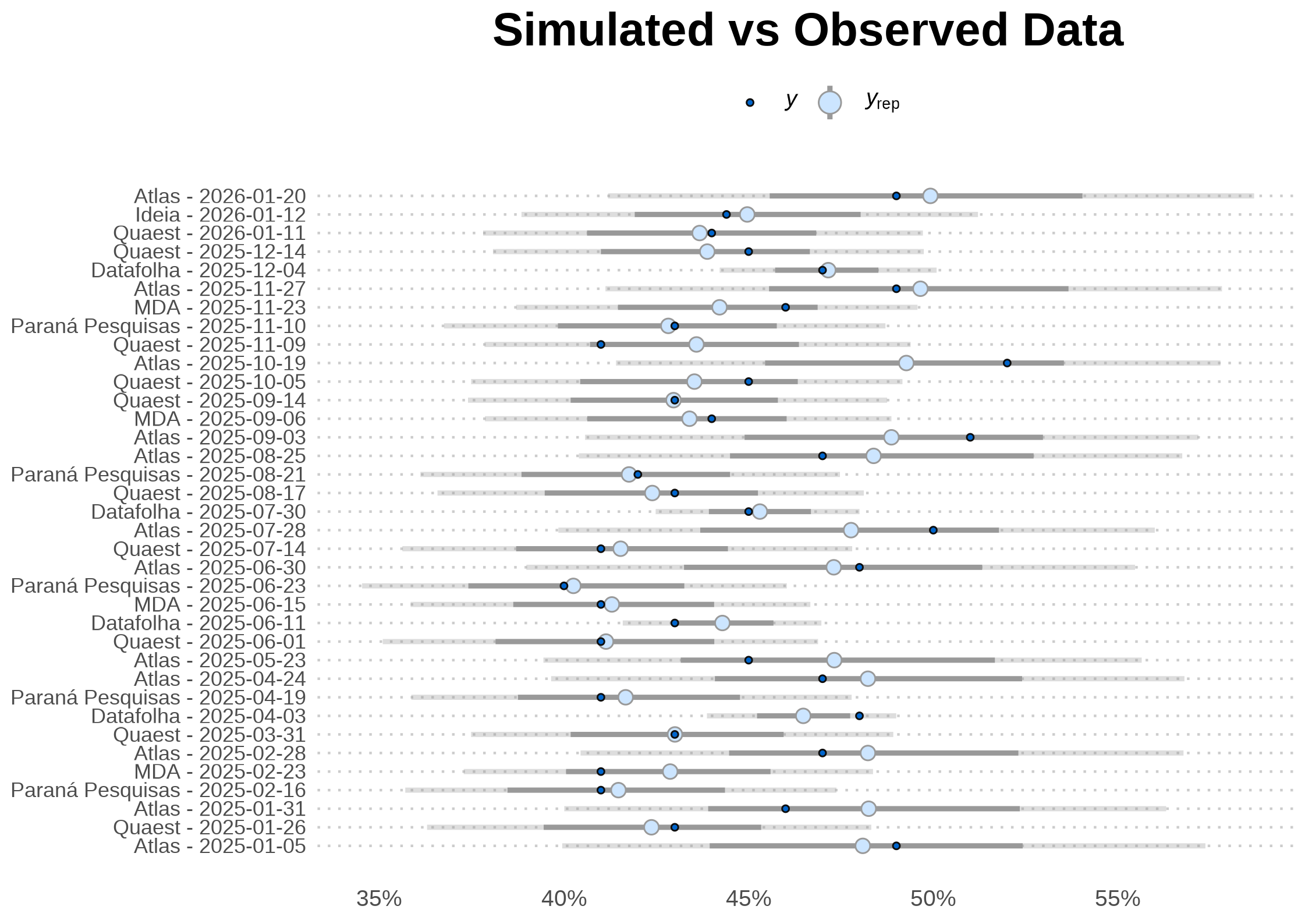
Parameter distributions are standardized using Non-Centered Parametrization (Stan Development Team, Efficiency Tuning: Reparametrization). This flattens posterior geometry and addresses the “funnel” problem common in hierarchical models (Gabry et al., 2019), significantly improving sampling efficiency and virtually eliminating divergent transitions in standard scenarios.
# Posterior geometry for selected mu and delta parameters
mcmc_scatter(modelo_cand$draws(),
             pars = c("mu[1]", "delta[1]"),
             np = nuts_params(modelo_cand), # no divergences to display
             alpha = 0.1) +
  stat_density_2d(color = "black")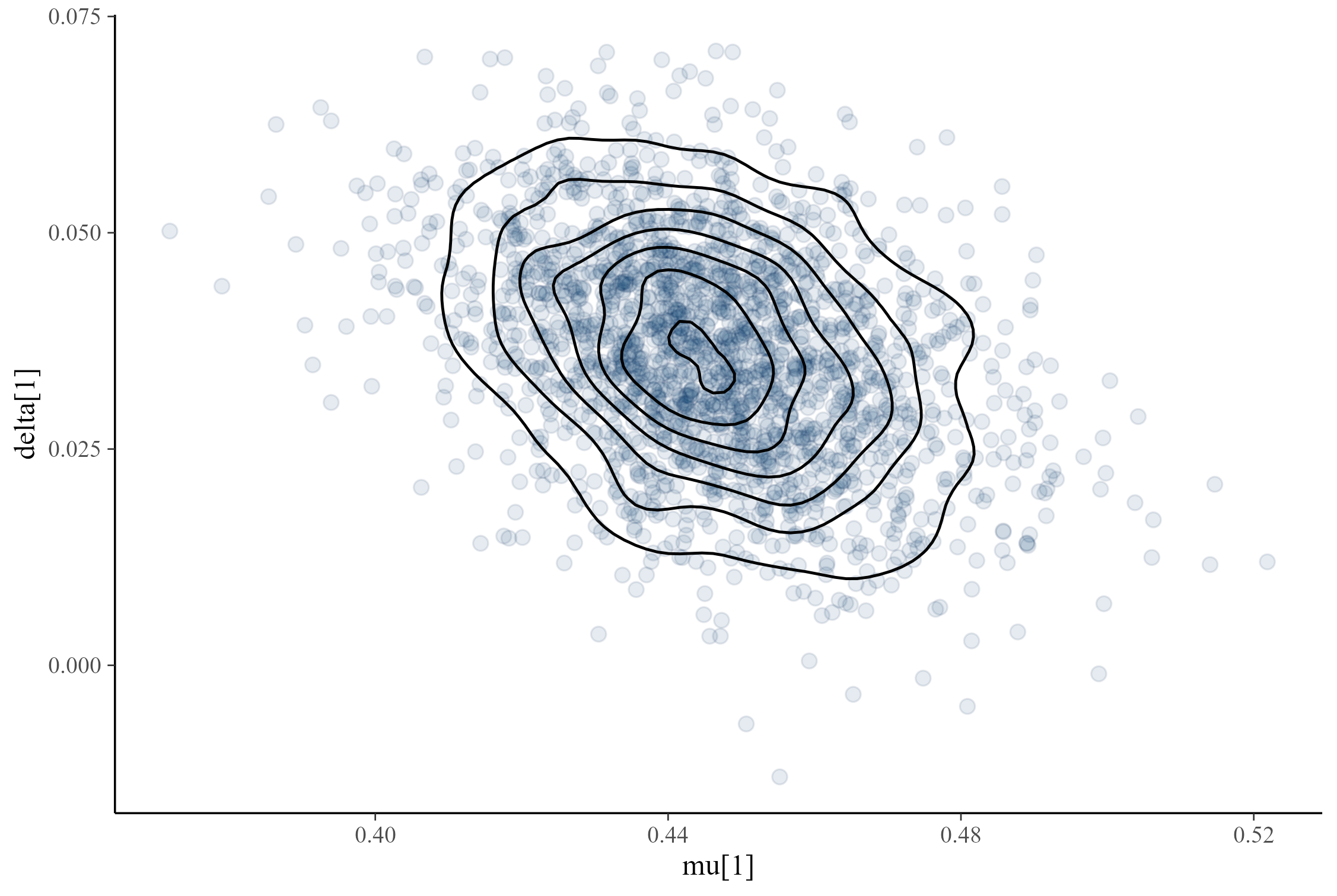
High sampling efficiency allows for fast models without sacrificing inference quality. Typical values for Effective Sample Size (ESS) and R-hat fall comfortably within recommended benchmarks. Notably, many parameters exhibit an ESS exceeding the nominal number of post-warmup iterations (blue line).
# ESS (bulk) vs R-hat
ggplot(modelo_cand$summary(), aes(x = ess_bulk, y = rhat)) +
  geom_point(alpha = 0.3) +
  geom_hline(yintercept = 1.01, linetype = "dashed", color = "red") +
  geom_vline(xintercept = 400, linetype = "dashed", color = "red") +
  geom_vline(xintercept = 2000, linetype = "dashed", color = "blue") +
  labs(title = "Convergence Diagnostics",
       subtitle = "Reference values: R-hat < 1.01 | ESS (bulk) > 4 x 100 | Iterations (post-warmup): 4 x 500)",
       x = "Effective Sample Size (bulk)",
       y = "R-hat") +
  theme_minimal() +
  theme(text = element_text(family = "Fira Sans"),
        plot.title = element_text(face = "bold", size = 18, hjust = .5),
        plot.subtitle = element_text(hjust = .5, color = "#777777"))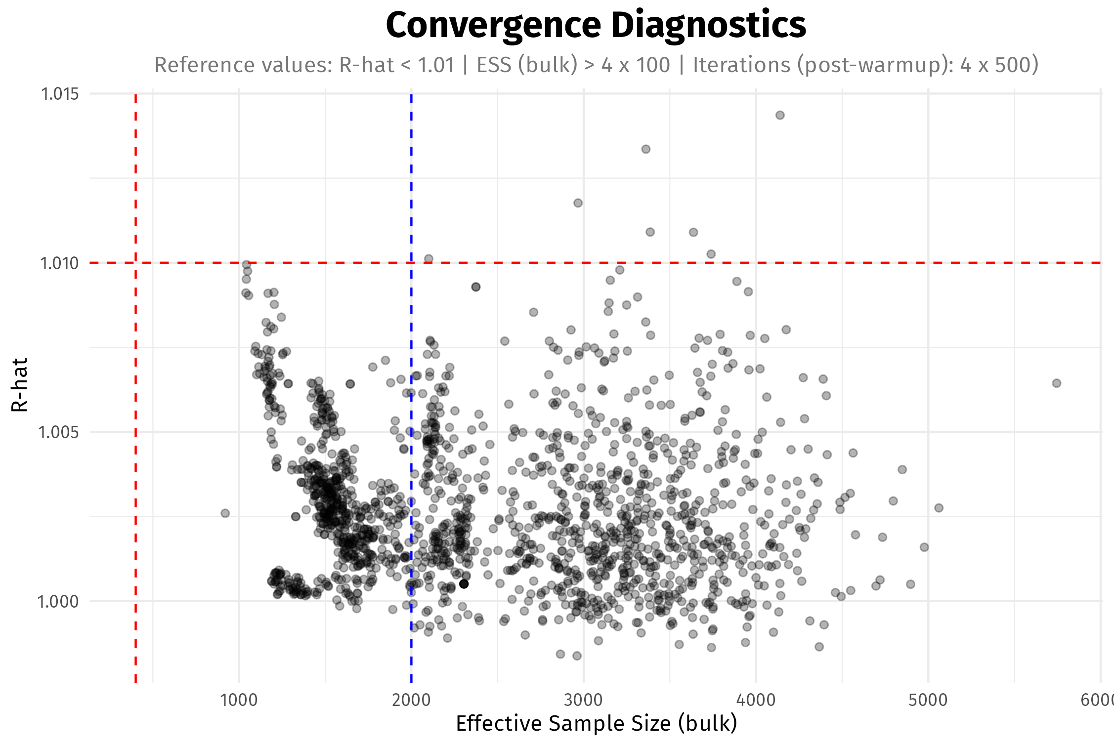
Gabry, J., Simpson, D., Vehtari, A., Betancourt, M., & Gelman, A. (2019). Visualization in Bayesian Workflow. Journal of the Royal Statistical Society Series A: Statistics in Society.
Heidemanns, H., Gelman, A., & Morris, G. (2020). An Updated Dynamic Bayesian Forecasting Model for the 2020 Election. Harvard Data Science Review.
Jackman, S. (2009). Bayesian Analysis for the Social Sciences. Wiley.
Stan Development Team. Stan User’s Guide (Efficiency Tuning: Reparametrization). Retrieved from https://mc-stan.org/docs/stan-users-guide/efficiency-tuning.html#reparameterization.section
Stoetzer, L. F., et al. (2019). Forecasting Elections in Multiparty Systems: A Bayesian Approach Combining Polls and Fundamentals. Political Analysis.
Partial pooling struggles to identify group-level variances in low-information environments like early campaigns, often leading to complete shrinkage or convergence failures. Anchoring the scale parameters keeps the models robust and reliable throughout the entire cycle.↩︎