tipitaka

The goal of tipitaka is to allow students and researchers to apply the tools of computational linguistics to the ancient Buddhist texts known as the Tipitaka or Pali Canon.

The Tipitaka is the canonical scripture of Theravadin Buddhists worldwide. It purports to record the direct teachings of the historical Buddha. It was first recorded in written form in what is now Sri Lanka, likely around 100 BCE.

The tipitaka package provides the texts of the Tipitaka in various electronic forms, plus functions for working with the Pali language.

Related Packages

For a lemmatized critical edition of the Tipitaka with sutta-level granularity, see tipitaka.critical.

Data Sources

This package includes the complete Tipitaka from the Chattha Sangayana Tipitaka version 4.0 (CST4) published by the Vipassana Research Institute. It covers all three pitakas (Vinaya, Sutta, and Abhidhamma).

• tipitaka_raw — Full text per volume (shipped as data)
• tipitaka_long — Word frequencies per volume (computed on first access)
• tipitaka_wide — Word frequency matrix (computed on first access)

Pali Alphabet

There is no universal script for Pali; traditionally each Buddhist country uses its own script to write Pali phonetically. This package uses the Roman script and the diacritical system developed by the PTS. However, note that the Pali alphabet does NOT follow the alphabetical ordering of English or other Roman-script languages. For this reason, tipitaka includes pali_alphabet giving the full Pali alphabet in order, and the functions pali_lt, pali_gt, pali_eq, and pali_sort for comparing and sorting Pali strings.

Installation

You can install the released version of tipitaka from CRAN with:

install.packages("tipitaka")

And the development version from GitHub with:

# install.packages("devtools")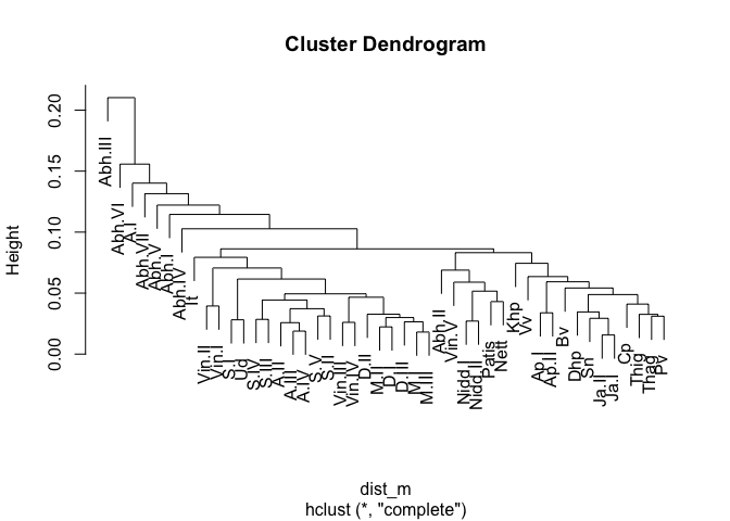
devtools::install_github("dangerzig/tipitaka")

Example

You can use tipitaka to do clustering analysis of the various books of the Pali Canon. For example:

library(tipitaka)
dist_m <- dist(tipitaka_wide)
cluster <- hclust(dist_m)
plot(cluster)

You can also create traditional k-means clusters and visualize these using packages like factoextra:

library(factoextra) # great visualizer for clusters
km <- kmeans(dist_m, 2, nstart = 25, algorithm = "Lloyd")
fviz_cluster(km, dist_m, labelsize = 12, repel = TRUE)

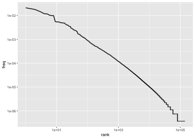
Finally, we can look at word frequency by rank:

library(dplyr, quietly = TRUE)
freq_by_rank <- tipitaka_long %>%
  group_by(word) %>%
  add_count(wt = n, name = "word_total") %>%
  ungroup() %>%
  distinct(word, .keep_all = TRUE) %>%
  mutate(tipitaka_total =
           sum(distinct(tipitaka_long, book,
                        .keep_all = TRUE)$total)) %>%
    transform(freq = word_total/tipitaka_total) %>%
  arrange(desc(freq)) %>%
  mutate(rank = row_number()) %>%
  select(-n, -total, -book)

freq_by_rank %>%
  ggplot(aes(rank, freq)) +
  geom_line(size = 1.1, alpha = 0.8, show.legend = FALSE) +
  scale_x_log10() +
  scale_y_log10()